coursera-data-engineering
Week 4 Lab 2:
Airflow 101 - Best Practices
In this lab, you will apply some of the best practices in orchestrating data pipelines in Airflow. You will build two DAGs that extract data from an RDS database, transform it and load it into a storage service. After this lab, you’ll be able to:
- Implement variables and templating in an Airflow DAG following best practices
- Integrate cross-communication between Airflow Tasks using XCOMs
- Organize Airflow Tasks into groups to improve DAG readability and monitoring
If you get stuck with completing the code in the exercises, you can download the solution files by running the following command in your Cloud9 environment:
aws s3 cp --recursive s3://dlai-data-engineering/labs/c2w4lab2-547818-solution/ ./
In case your Apache Airflow environment presents any issues, you can always restart it by running the following bash script:
bash ./scripts/restart_airflow.sh
This process will end when the service is healthy. That should take less than 3 minutes.
1 - Best Practices in Writing DAGs
In this first section, we will review some of the best practices in writing DAGs in Airflow, which you’ve already seen in the video tutorials or the reading items of this lesson. In the remaining sections, you will apply those practices in Airflow. Feel free to directly start with the second section, if those practices are still fresh in your mind.
1.1 - Determinism and Idempotence
Airflow best practices help you write reproducible, efficient and reliable code, appropriately share data between tasks and reduce the time to recover from a data downtime. Determinism and Idempotence, which are essential concepts in Data Engineering, are the basis for reproducible and reliable data pipelines. Determinism means that the same input will always produce the same output. Idempotence means if you execute the same operation multiple times, you will obtain the same result.
In Airflow, you can achieve determinism and idempotence by correctly defining your DAGs and tasks, using built-in Airflow variables, and building parameterized operators. When defining your DAG, there are several parameters that you can specify to manage your DAG execution and ensure that it is deterministic and idempotent. The following are the most important ones:
- The
scheduleparameter: defines the frequency at which the DAG will be executed. - The
start_dateparameter: defines the start date of the first data interval. The start date should be static to avoid missing DAG runs and prevent confusion; static date means a fixed date likedatetime.datetime(2024, 5, 20). - The
catchupparameter: defines whether the DAG will be executed for all the data intervals between thestart_dateand the current date. It is recommended that you set it toFalseto have more control over the execution of the DAG. You can also use the [Backfill] (https://airflow.apache.org/docs/apache-airflow/stable/dag-run.html#backfill) feature to execute the DAG for a specific date range.
1.2 - Built-in Variables and Templating
Templating allows Airflow tasks to dynamically evaluate information at runtime and use it to execute tasks. You can use templating to dynamically evaluate either user-created variables or built-in Airflow variables. The templating syntax is ``. You can find more information about templating in the Airflow documentation.
An advantage of Airflow templating is that it leverages the power of Jinja Templating, as it uses double curly braces `` to retrieve the information, avoiding the need to write top-level code in your DAG file.
Airflow provides a set of built-in variables that you can use to retrieve information about the execution of your DAG. For
example, you can use the `` variable to retrieve the DAG run’s logical
date as YYYY-MM-DD. In this way, your specific DAG run will be able to
retrieve the information detailed to its execution and achieve determinism.
You can also use Macros to transform or format the built-in variables, for
example, you could change the format of the `` variable using the
macros.ds_format function. You can find more documentation here.
1.3 - User-Created Variables
Hard-coded and duplicated values can harm your DAG. Updating those values in multiple places can be tedious and open the door for errors. To avoid this unnecessary burden and follow the Don’t Repeat Yourself (DRY) principle, a best practice is to use user-created variables, allowing you to store, update, retrieve and delete key-value content to be used dynamically by your DAG.
To access a user-created variable inside the DAG, you can use this example:
from airflow.models import Variable
foo = Variable.get("foo")
1.4 - XCOMs
Airflow tasks are executed independently but sometimes you need to share information between the tasks. For example, you might need to pass information from one task to another task, or you might have to gather information from a previous task. In these cases, you can use XCOMs to share information between tasks.
An XCOM is identified by a key, as well as the task_id and dag_id where it
came from. They are stored using the xcom_push method and retrieved using the
xcom_pull method inside the task. But, many operators will automatically
push their results into an XCOM key called return_value.
Because XCOMs are stored in the Airflow metadata database by default, you should not use them to store large amounts of data as they can harm the performance of your Airflow database. Instead, you can use them to store small pieces of information that you need to share between tasks.
# Pushing an XCom
context['ti'].xcom_push(key='data_key', value=data)

# Pulling an XCom
data = context['ti'].xcom_pull(key='data_key', task_ids='task_id')
1.5 - Task Groups
In Airflow, you can group tasks using Task Groups. Task Groups allow you to
group tasks in the Airflow UI, organize your DAGs and make them more readable.
Inside the task group, you can define tasks and the dependencies between them
using the bit-shift operators << and >>. You can create a Task Group using
the with statement, as shown in the following example.
from airflow.utils.task_group import TaskGroup

with DAG(...):
    start = DummyOperator(...)

    task_group = []
    with TaskGroup(...) as etl_tg:
        task_a = PythonOperator(...)

        task_b = PythonOperator(...)

        task_a >> task_b

        # append each of the `etl_tg` elements into the `task_group`
        task_group.append(etl_tg)

    end = DummyOperator(...)

    start >> task_group >> end
Note: This lab uses
pandasto transform the data within the Airflow instance. This is done for educational purposes. It is not desirable in real-life Airflow pipelines for the following two reasons:
- Airflow should interact with storage and processing solutions using operators specifically designed for them.
- Airflow should only be an orchestrator, and it should delegate the actual processing the workload of the pipeline to the appropriate tools such as databases or Spark clusters.
This is a BAD practice, but one that would help here to show you the best practices in other aspects of Airflow.
2 - Exploring Airflow’s Components and Lab Resources
For this lab, you are provided with a MySQL database that represents the
source system you will interact with. The database classicmodels (MySQL Sample Database) is already instantiated for you in Amazon RDS.
You have used this database in the previous labs. In this lab, you will interact
with 4 of its tables: orders, customers , payments and products to
create two DAGs. If you need to review how to access the database, you can read
the instructions in the last (optional) section of this lab.
You are provided with a dockerized version of Airflow that is running on an EC2 instance. You will only need to interact with the Airflow UI and the S3 bucket that represents the DAG directory, not with the EC2 instance directly.
2.1. To access your Airflow UI, go to the AWS console and search for
CloudFormation. You will see two stacks deployed, one associated with your
Cloud9 environment (name with prefix aws-cloud9) and another named with an
alphanumeric ID. Click on the alphanumeric ID stack and search for the
Outputs tab. You will see the key AirflowDNS with the complete URL to
access the Airflow UI in the Value column. Copy it and paste it into another
browser tab. You will see a login page, use the following credentials:
- username:
airflow - password:
airflow
Note: It might happen that you won’t see a login screen straight away. As the Airflow’s components deployment can take several minutes, it is possible that the first time you copy the URL, the service will not be yet available. You can continue working on the following exercises in Cloud9 and refresh the Airflow UI tab in a few minutes to see the login screen.
2.2. Review the CloudFormation Outputs of the deployed stack. There are other values that you will need for the lab.
Similarly to the previous lab, you’ll use Raw Data Bucket to write code, create and delete files, and DAGs Bucket to upload the Python scripts defining your DAGs (which will be recognized by Airflow). Check the names of those two buckets in the CloudFormation Outputs.
3 - Building a Simple DAG
You will use the following DAG which comprises five tasks to process the orders
table from classicmodels.
3.1 - DAG Structure

Here are the descriptions of the DAG tasks:
-
start: is an empty task marking the start of the DAG. Here you will useDummyOperator. Similarly toEmptyOperatorit doesn’t include any behavior, but it creates a task instance in the Airflow metadata database. extract_load_orders: extracts data from the tableordersand loads it into a zone in the S3 bucket (bronze zone), using the following destination path:s3://<BUCKET_NAME>/bronze/orders/YYYY/MM/DD/You will implement this task using the SqlToS3Operator. It is an Amazon transfer operator, which you can use to copy data from a SQL server to an S3 file.
transform_orders: transforms the data extracted from the tableordersand loads it into another zone of the S3 bucket (silver zone), using the following destination path:s3://<BUCKET_NAME>/silver/orders/YYYY/MM/DD/The transformation consists of dropping the null records and duplicate rows from the table
orders. You will execute this task using thePythonOperatorthat calls thedrop_nas_and_duplicatesfunction.-
notification: emulates a notification task that sends an email with the number of the resultant records in the transformed table. In this lab, this task will just print the number of rows of the transformed data. You will execute this task using thePythonOperatorthat calls thenotify_valid_recordsfunction. end: is an empty task marking the end of the DAG. It doesn’t include any behavior and will be executed also with theDummyOperator.
Note that in this lab, the functions drop_nas_and_duplicates and
notify_valid_records are defined outside the DAG definition, at the start of
the Python script.
3.2 - Preparing the Python Code
In this section, you will need to complete the Python script simple_dag.py,
which you can find in the folder src/ Once you’re done, you’ll upload the
file to the appropriate bucket and manually trigger the DAG in the Airflow UI.
Exercise 1
Complete the definitions of the DAG in src/simple_dag.py, in the section
associated with EXERCISE 1. The DAG should have the following characteristics:
- run daily;
- a static start date using the
datetimeobject. You can specify the date at which you’re doing the lab; - not run for past dates.
Note: To start exercise 1, you need to scroll down to get to the with
statement where the DAG is instantiated.
Exercise 2
In this exercise, you will use the ds variable to retrieve the DAG run’s
logical date (see Section 1.2 above). You will use this information to define
the destination path in S3, for the data you will extract and load from the
orders table. This way, when the same DAG runs for different data intervals,
the extracted data will be organized in S3 according to the date it belongs to.
We will refer to this date as the S3 partition date.
Define the partition_date variable in src/simple_dag.py file, in the section
associated with EXERCISE 2. The partition_date should be in the YYYY/MM/DD
format.
Exercise 3
Airflow has the concept of Connection that you can use to store credentials that enable your DAG to
connect to external systems. A connection consists of a set of parameters - such
as login, password and hostname - along with the connection type and connection
Id. You can create a connection in the Airflow UI and then use the connection
ID in your code. In this exercise, you will create a connection that contains
the values of the parameters needed to connect to the MYSQL database and then pass
the connection ID to SqlToS3Operator.
- Create a connection in the Airflow UI: select the Admin tab in the
header, then select the Connections option.
Click the add button + and complete the connection with the following
values:
Connection Id: A unique identifier for the connection, e.g.mysql_connection.Connection type: SelectMySQLfrom the dropdown menu (you may need to scroll down through the list).Host: Endpoint of the RDS database. One of the CloudFormation stack outputs.Schema: The schema name of the RDS database. In this case, it isclassicmodels. (See optional section below: when you connect to MySQL RDS, you can run the commandshow databasesto get the schema or database name).Login: The user for the RDS database. You can find it in the CloudFormation stack tab Parameters, value for the keyDatabaseUserName.Password: The password for the user in the RDS database. In this case, it isadminpwrd.Port: The port for the RDS database. In your case,3306is the default port for MySQL.
This is an example of how the Connection creation should look like:
 .
.Click on Save.
- Create a variable in the Airflow UI: select the Admin tab in the header,
then select the Variables option.
Click the add button + and complete the variable with the following
values:
Key:s3_bucket,Val: name of the Raw Data Bucket.
Click on Save.
-
Complete the definition of the
extract_load_orderstask, which usesSqlToS3Operator. Follow the instructions in the section. When you get to the SQL query part, you need to write a SQL statement to retrieve all the data from theorderstable:SELECT * FROM orders;
Exercise 4
Complete the function drop_nas_and_duplicates in the src/simple_dag.py file,
in the section associated with EXERCISE 4 (at the start of the script). This
function includes the transformation steps, where you can use pandas to do
basic data cleaning - detecting null rows and dropping duplicate rows.
Exercise 5
Complete the transform_orders task in the src/simple_dag.py file, in the
section associated with EXERCISE 5 using the drop_nas_and_duplicates
function you defined in the previous exercise.
The transform_orders task is in charge of dropping nulls and duplicate rows
from the orders table, which you loaded into the S3 bucket in Exercise 3.
After that, the same task will store the transformed data back to S3. This task
will also push the number of rows left after the transformation into an XCOM.
Exercise 6
Complete the function notify_valid_records in the src/simple_dag.py file, in
the section associated with EXERCISE 6 (at the start of the script). Use XCOM
pull to extract the value pushed from the transform_orders task.
Exercise 7
Complete the notification task in the src/simple_dag.py file, in the section
associated with EXERCISE 7. Use the function notify_valid_recordsyou
defined in exercise 6.
Exercise 8
Finish the DAG by completing the task dependencies at the end of the file, use
the bit-shift operators >> to define the relation between the tasks. When you
load your DAG in the Airflow UI, the DAG should look like the DAG visualized in
section 3.
4 - Running Your DAGs with Airflow
After you’ve finished all the exercises, the simple_dag.py file should be
ready to be uploaded to the DAG directory. To upload your file to the
DAGs Bucket, remember first to save any changes or updates to
simple_dag.py and then use the following command from the Cloud9 terminal:
aws s3 sync src s3://<DAGS-BUCKET>/dags
Once the environment has finished syncing the content of the buckets (remember it can take up to 10 minutes), go to the Airflow UI. Keep refreshing the web interface, and after a couple of minutes, you should see that it recognizes your simple DAG. You will also get an error with loading the second DAG. Don’t worry about it, as you’re going to complete the second DAG in the next section.
Now activate (unpause) the simple DAG and trigger the DAG manually with the run button on the right. If the tasks didn’t succeed, use the logs to find the problem and return to the corresponding script to correct it.
If your runs didn’t succeed the first time, and you have already detected and corrected the source of the problem, go back to Airflow’s web interface and navigate to the Grid view page. There you can rerun the failed tasks so that Airflow performs them again. When you get successful runs, go to the Raw Data Bucket (not the DAGs Bucket) to see if the appropriate files were created.
5 - Grouped Tasks DAG
5.1 - DAG Structure
Here is the second DAG you will set up:

-
start: is an empty task marking the start of the DAG. It doesn’t include any behavior. -
extract_load_<table>: extracts data from the table<table>and loads it into the S3 bucket (Raw Data Bucket). The destination path iss3://<BUCKET_NAME>/bronze/<table>/YYYY/MM/DD/. You will execute this task using the SqlToS3Operator. -
transform_<table>: transforms the data extracted from the table<table>and loads it into another zone of the S3 bucket. The destination path iss3://<BUCKET_NAME>/silver/<table>/YYYY/MM/DD/. The transformation also consists of dropping the null records and duplicate rows. You will also use aPythonOperatorwhich will call thedrop_nas_and_duplicatesfunction.
The remaining tasks send_notificationand end are similar to the tasks you
implemented in the first DAG. Note that the task send_notification will print
the number of the resultant records of each table.
For this set of exercises, you have to complete the TaskGroups required to
extract, load, and transform the payments, customers and products tables
from the classicmodels dataset in the src/grouped_task_dag.py.
5.2 - Preparing the Python Code
Exercise 9
Go through the code in the file src/grouped_task_dag.py to check the
components of the tasks. Find the section related to Exercise 9 and complete
the code, defining the dependency between the task extract_load and
transform. Then append the tasks into the task_group variable.
Exercise 10
Finish the DAG by completing the task dependencies at the end of the file, use
the bit-shift operators >>. It should look like the DAG visualized in the section
5.1. Follow the instructions in 4 - Running Your DAGs with Airflow section to
test the DAG script.
In this lab, you have implemented an idempotent and deterministic DAG, applying several best practices. You have used templating and variables to dynamically retrieve information and avoid hard-coded and duplicated values. You have also used XCOMs to share data between tasks and Task Groups to organize your DAGs and make them more readable.
6 - Optional material
Here is some information about the classicmodels database. It contains typical
business data about classic car retailers, including information about
customers, products, sales orders, sales order line items, and more; however,
you will only be working with the following tables:
orders: Contains information about orders placed by customers, including the status and significant dates of the process.customers: Contains basic information about customers, such as their name, phone, and location.products: Contains information about products, including the name, product line, and price.
Here are the steps to connect to the database and explore the data:
6.1. Get the endpoint of the database instance in the CloudFormation Outputs.
6.2. Now connect to the database by running the following command, replacing
<MySQLEndpoint> with the output from the previous step:
mysql --host=<MySQLEndpoint> --user=admin --password=adminpwrd --port=3306
You will access MySQL monitor which gives visibility into the performance and availability of the instance.
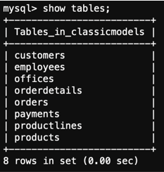
6.3. Now that you checked the existence of the Amazon RDS MySQL instance, you can verify that the data exists within the database:
use classicmodels;
show tables;
You should get an output similar to this one:
6.4. Enter exit in the terminal to quit the database connection.
exit