coursera-data-engineering

Data Transformations with Apache Spark

In this lab, you will perform transformations on the classicmodels database with Apache Spark. You will learn the basics and then create a star schema model similar to the one done in the Week 1 assignment.

1 - Introduction
2 - Environment Setup
3 - Apache Spark 101
4 - Data Modeling with Spark
5 - Upload Files for Grading

1 - Introduction

Apache Spark is an open-source unified analytics engine for large-scale data processing, it allows you to perform Data Engineering, Data Science, and Machine Learning jobs on single-node machines or clusters. During the courses you have seen some examples with AWS Glue jobs, a serverless service that allows you to run Spark jobs without setting up cloud resources. In this particular assignment, you will use Amazon EMR to run a Spark cluster and use its Studio and Workspace functions to run jobs from this notebook directly on top of the cluster.

You will recreate the Star Schema data model from the Week 1 assignment using PySpark, a Python API for Spark.

2 - Environment Setup

The classicmodels database is stored in an RDS instance running a Postgres engine, you will need to configure the connection to read the source data and then store the generated data models. Thankfully, the Studio functionality of Amazon EMR provides you with the necessary classes ready to use, but you will need to add a configuration to allow the environment to connect to a Postgres database.

2.1. Run the following cell, this will point the Spark cluster to a JAR file with the necessary code to connect:

%%configure -f
{
    "conf": {
        "spark.pyspark.python": "python",
        "spark.pyspark.virtualenv.enabled": "true",
        "spark.pyspark.virtualenv.type":"native",
        "spark.pyspark.virtualenv.bin.path":"/usr/bin/virtualenv",
        "spark.jars.packages": "org.postgresql:postgresql:42.2.5"
    }
}

Current session configs: {‘conf’: {‘spark.pyspark.python’: ‘python’, ‘spark.pyspark.virtualenv.enabled’: ‘true’, ‘spark.pyspark.virtualenv.type’: ‘native’, ‘spark.pyspark.virtualenv.bin.path’: ‘/usr/bin/virtualenv’, ‘spark.jars.packages’: ‘org.postgresql:postgresql:42.2.5’}, ‘proxyUser’: ‘assumed-role_voclabs_user122191_Piyush_Patel’, ‘kind’: ‘pyspark’}

No active sessions.

2.2. Go to CloudFormation in the AWS console. You will see the stack with an alphanumeric ID. Click on it and search for the Outputs tab. You will see the key PostgresEndpoint, copy the corresponding Value (highlight and copy it as text, not as a link). Replace the placeholder <RDS-ENDPOINT> in the following cell and run it.

RDS_ENDPOINT = "de-c4w3a1-rds.cbesi8oiibou.us-east-1.rds.amazonaws.com"
jdbc_url = f"jdbc:postgresql://{RDS_ENDPOINT}:5432/postgres"  # For PostgreSQL

jdbc_properties = {
    "user": "postgresuser",
    "password": "adminpwrd",    
    "driver": "org.postgresql.Driver"  # For PostgreSQL
}

VBox()

Starting Spark application

ID	YARN Application ID	Kind	State	Spark UI	Driver log	User	Current session?
0	application_1727634572160_0001	pyspark	idle	Link	Link	None	✔

FloatProgress(value=0.0, bar_style='info', description='Progress:', layout=Layout(height='25px', width='50%'),…

SparkSession available as 'spark'.

FloatProgress(value=0.0, bar_style='info', description='Progress:', layout=Layout(height='25px', width='50%'),…

After running the previous cell you should wait while the Spark application starts. After it finishes, you should see a message like this:

SparkSession available as 'spark'

2.3. Now use the spark object that is available to read from the database using Java Database Connectivity (JDBC), you will provide the JDBC url and the connection properties, and point to a table with their corresponding schema. In this case, you will call information_schema.tables to get the available tables; then you will select the schema and names.

%%pyspark
information_tables_df = spark.read.jdbc(jdbc_url, "information_schema.tables", properties=jdbc_properties)
information_tables_df.select(["table_schema", "table_name"]).show()

FloatProgress(value=0.0, bar_style='info', description='Progress:', layout=Layout(height='25px', width='50%'),…


+-------------+--------------------+
| table_schema|          table_name|
+-------------+--------------------+
|classicmodels|           employees|
|classicmodels|             offices|
|classicmodels|           customers|
|classicmodels|        orderdetails|
|classicmodels|        productlines|
|classicmodels|            products|
|classicmodels|              orders|
|   pg_catalog|             pg_type|
|classicmodels|            payments|
|   pg_catalog|    pg_foreign_table|
|   pg_catalog|            pg_roles|
|   pg_catalog|         pg_settings|
|   pg_catalog|pg_shmem_allocations|
|   pg_catalog|pg_backend_memory...|
|   pg_catalog|    pg_stat_activity|
|   pg_catalog|     pg_subscription|
|   pg_catalog|        pg_attribute|
|   pg_catalog|             pg_proc|
|   pg_catalog|            pg_class|
|   pg_catalog|          pg_attrdef|
+-------------+--------------------+
only showing top 20 rows

2.4. Now that you listed the available schemas, call the information_schema.schemata table. Select the schema_name and schema_owner, and then show the resulting dataframe.

information_schemas_df = spark.read.jdbc(jdbc_url, "information_schema.schemata", properties=jdbc_properties)
information_schemas_df.select(["schema_name", "schema_owner"]).show()

VBox()



FloatProgress(value=0.0, bar_style='info', description='Progress:', layout=Layout(height='25px', width='50%'),…


+--------------------+-----------------+
|         schema_name|     schema_owner|
+--------------------+-----------------+
|              public|pg_database_owner|
|       classicmodels|     postgresuser|
|         test_schema|     postgresuser|
|classicmodels_sta...|     postgresuser|
|  information_schema|         rdsadmin|
|          pg_catalog|         rdsadmin|
+--------------------+-----------------+

3 - Apache Spark 101

As mentioned before, Apache Spark is a workload engine that can be used with high-level APIs in programming languages such as Java, Scala and Python. The core abstraction of Spark is a Resilient Distributed Dataset (RDD), which is a collection of elements that can be partitioned across the nodes of the cluster; this enables running intensive workloads on the data in parallel. Spark also has some high-level toolsets like Spark SQL for structured data processing using SQL, pandas API for Spark to run pandas workloads, and MLlib for machine learning workloads.

You will focus on PySpark, the Python API. However, you will skip the details on how to connect to a Spark cluster and most of the initial setup required as the necessary configuration to run this notebook has already been provided. You will get a brief overview of the required classes to access Spark with PySpark and run our workloads.

3.1 - Spark Classes

To start a Spark program you must create a SparkConf object, that contains information about your application, and a SparkContext object, which tells Spark how to access a cluster.

from pyspark import SparkContext, SparkConf
conf = SparkConf().setAppName(appName).setMaster(master)
sc = SparkContext(conf=conf)

The appName parameter is a string with the name of your application, it shows on the Spark cluster UI. master is the connection string to a Spark cluster or a "local" string to run in local mode.

3.2 - Spark Dataframe

In this lab you will be using the PySpark DataFrame API, the API enables the use of Spark Dataframes, an abstraction on top of RDDs. For PySpark applications running this API, you can start by initializing a SparkSession object which is the entry point of PySpark.

from pyspark.sql import SparkSession

spark = SparkSession.builder.getOrCreate()

In this notebook, you can access a preconfigured SparkSession object using the spark variable, you have used before to read the available tables. Now, you will start looking into the Spark dataframe. Let’s read the orders table from the classicmodels schema.

%%pyspark

# Read data from RDS into a Spark DataFrame
orders_df = spark.read.jdbc(url=jdbc_url, table="classicmodels.orders", properties=jdbc_properties)

FloatProgress(value=0.0, bar_style='info', description='Progress:', layout=Layout(height='25px', width='50%'),…

Let’s explore the dataframe operations available, here is a list of some of the most important ones:

df.printSchema(): Prints the schema of the dataframe.
df.select("col"): Select the column of the name col from the dataframe.
df.show(): Prints the content of the dataframe.
df.filter(df["col"] > value): Filters the dataframe based on a logical condition.
df.groupBy("col").agg(): Perform an aggregation based on a column of name col. The aggregation can be count, max, min, avg.
df.withColumn("new_col",col_values): Adds a new column to the dataframe with the new_col name and col_values as values for the column.

Let’s start by printing the content of the orders dataframe.

orders_df.show()

VBox()



FloatProgress(value=0.0, bar_style='info', description='Progress:', layout=Layout(height='25px', width='50%'),…


+-----------+-------------------+-------------------+-------------------+-------+--------------------+--------------+
|ordernumber|          orderdate|       requireddate|        shippeddate| status|            comments|customernumber|
+-----------+-------------------+-------------------+-------------------+-------+--------------------+--------------+
|      10100|2003-01-06 00:00:00|2003-01-13 00:00:00|2003-01-10 00:00:00|Shipped|                NULL|           363|
|      10101|2003-01-09 00:00:00|2003-01-18 00:00:00|2003-01-11 00:00:00|Shipped|Check on availabi...|           128|
|      10102|2003-01-10 00:00:00|2003-01-18 00:00:00|2003-01-14 00:00:00|Shipped|                NULL|           181|
|      10103|2003-01-29 00:00:00|2003-02-07 00:00:00|2003-02-02 00:00:00|Shipped|                NULL|           121|
|      10104|2003-01-31 00:00:00|2003-02-09 00:00:00|2003-02-01 00:00:00|Shipped|                NULL|           141|
|      10105|2003-02-11 00:00:00|2003-02-21 00:00:00|2003-02-12 00:00:00|Shipped|                NULL|           145|
|      10106|2003-02-17 00:00:00|2003-02-24 00:00:00|2003-02-21 00:00:00|Shipped|                NULL|           278|
|      10107|2003-02-24 00:00:00|2003-03-03 00:00:00|2003-02-26 00:00:00|Shipped|Difficult to nego...|           131|
|      10108|2003-03-03 00:00:00|2003-03-12 00:00:00|2003-03-08 00:00:00|Shipped|                NULL|           385|
|      10109|2003-03-10 00:00:00|2003-03-19 00:00:00|2003-03-11 00:00:00|Shipped|Customer requeste...|           486|
|      10110|2003-03-18 00:00:00|2003-03-24 00:00:00|2003-03-20 00:00:00|Shipped|                NULL|           187|
|      10111|2003-03-25 00:00:00|2003-03-31 00:00:00|2003-03-30 00:00:00|Shipped|                NULL|           129|
|      10112|2003-03-24 00:00:00|2003-04-03 00:00:00|2003-03-29 00:00:00|Shipped|Customer requeste...|           144|
|      10113|2003-03-26 00:00:00|2003-04-02 00:00:00|2003-03-27 00:00:00|Shipped|                NULL|           124|
|      10114|2003-04-01 00:00:00|2003-04-07 00:00:00|2003-04-02 00:00:00|Shipped|                NULL|           172|
|      10115|2003-04-04 00:00:00|2003-04-12 00:00:00|2003-04-07 00:00:00|Shipped|                NULL|           424|
|      10116|2003-04-11 00:00:00|2003-04-19 00:00:00|2003-04-13 00:00:00|Shipped|                NULL|           381|
|      10117|2003-04-16 00:00:00|2003-04-24 00:00:00|2003-04-17 00:00:00|Shipped|                NULL|           148|
|      10118|2003-04-21 00:00:00|2003-04-29 00:00:00|2003-04-26 00:00:00|Shipped|Customer has work...|           216|
|      10119|2003-04-28 00:00:00|2003-05-05 00:00:00|2003-05-02 00:00:00|Shipped|                NULL|           382|
+-----------+-------------------+-------------------+-------------------+-------+--------------------+--------------+
only showing top 20 rows

You can create a Spark dataframe from collections such as a list of tuples, a list of dictionaries, an RDD, and a pandas dataframe. This is an example:

list_of_tuples = [("Alice", 1),("Bob", 2),("Carla", 3)]
spark.createDataFrame(list_of_tuples).show()

VBox()



FloatProgress(value=0.0, bar_style='info', description='Progress:', layout=Layout(height='25px', width='50%'),…


+-----+---+
|   _1| _2|
+-----+---+
|Alice|  1|
|  Bob|  2|
|Carla|  3|
+-----+---+

You can define the schema as a second parameter, either by passing a list of column names or a StructType, the later one uses an array of StructField for each column with the corresponding name, type and if the column accepts nulls.

from pyspark.sql.types import *
schema = StructType([
   StructField("name", StringType(), True),
   StructField("age", IntegerType(), True)])
test_df = spark.createDataFrame(list_of_tuples, schema)
test_df.show()

VBox()



FloatProgress(value=0.0, bar_style='info', description='Progress:', layout=Layout(height='25px', width='50%'),…


+-----+---+
| name|age|
+-----+---+
|Alice|  1|
|  Bob|  2|
|Carla|  3|
+-----+---+

Finally, you can also write Spark dataframes in the same formats that you can read. During this lab, you will save dataframes to the same database. Here is an example of how to store a dataframe to Postgres to a pre-created test_schema:

test_df.write.jdbc(url=jdbc_url, table="test_schema.test_table", mode="overwrite", properties=jdbc_properties)

VBox()

FloatProgress(value=0.0, bar_style='info', description='Progress:', layout=Layout(height='25px', width='50%'),…

3.3 - Spark SQL

As mentioned before, one of the high-level tools offerded by Spark is Spark SQL, this will be one of the main tools you will use during the lab. You can perform SQL queries using the available dataframes, first, you have to register each dataframe as a temporary view and then call the sql function from the SparkSession object.

orders_df.createOrReplaceTempView("orders")

sqlDF = spark.sql("SELECT * FROM orders")
sqlDF.show()

VBox()



FloatProgress(value=0.0, bar_style='info', description='Progress:', layout=Layout(height='25px', width='50%'),…


+-----------+-------------------+-------------------+-------------------+-------+--------------------+--------------+
|ordernumber|          orderdate|       requireddate|        shippeddate| status|            comments|customernumber|
+-----------+-------------------+-------------------+-------------------+-------+--------------------+--------------+
|      10100|2003-01-06 00:00:00|2003-01-13 00:00:00|2003-01-10 00:00:00|Shipped|                NULL|           363|
|      10101|2003-01-09 00:00:00|2003-01-18 00:00:00|2003-01-11 00:00:00|Shipped|Check on availabi...|           128|
|      10102|2003-01-10 00:00:00|2003-01-18 00:00:00|2003-01-14 00:00:00|Shipped|                NULL|           181|
|      10103|2003-01-29 00:00:00|2003-02-07 00:00:00|2003-02-02 00:00:00|Shipped|                NULL|           121|
|      10104|2003-01-31 00:00:00|2003-02-09 00:00:00|2003-02-01 00:00:00|Shipped|                NULL|           141|
|      10105|2003-02-11 00:00:00|2003-02-21 00:00:00|2003-02-12 00:00:00|Shipped|                NULL|           145|
|      10106|2003-02-17 00:00:00|2003-02-24 00:00:00|2003-02-21 00:00:00|Shipped|                NULL|           278|
|      10107|2003-02-24 00:00:00|2003-03-03 00:00:00|2003-02-26 00:00:00|Shipped|Difficult to nego...|           131|
|      10108|2003-03-03 00:00:00|2003-03-12 00:00:00|2003-03-08 00:00:00|Shipped|                NULL|           385|
|      10109|2003-03-10 00:00:00|2003-03-19 00:00:00|2003-03-11 00:00:00|Shipped|Customer requeste...|           486|
|      10110|2003-03-18 00:00:00|2003-03-24 00:00:00|2003-03-20 00:00:00|Shipped|                NULL|           187|
|      10111|2003-03-25 00:00:00|2003-03-31 00:00:00|2003-03-30 00:00:00|Shipped|                NULL|           129|
|      10112|2003-03-24 00:00:00|2003-04-03 00:00:00|2003-03-29 00:00:00|Shipped|Customer requeste...|           144|
|      10113|2003-03-26 00:00:00|2003-04-02 00:00:00|2003-03-27 00:00:00|Shipped|                NULL|           124|
|      10114|2003-04-01 00:00:00|2003-04-07 00:00:00|2003-04-02 00:00:00|Shipped|                NULL|           172|
|      10115|2003-04-04 00:00:00|2003-04-12 00:00:00|2003-04-07 00:00:00|Shipped|                NULL|           424|
|      10116|2003-04-11 00:00:00|2003-04-19 00:00:00|2003-04-13 00:00:00|Shipped|                NULL|           381|
|      10117|2003-04-16 00:00:00|2003-04-24 00:00:00|2003-04-17 00:00:00|Shipped|                NULL|           148|
|      10118|2003-04-21 00:00:00|2003-04-29 00:00:00|2003-04-26 00:00:00|Shipped|Customer has work...|           216|
|      10119|2003-04-28 00:00:00|2003-05-05 00:00:00|2003-05-02 00:00:00|Shipped|                NULL|           382|
+-----------+-------------------+-------------------+-------------------+-------+--------------------+--------------+
only showing top 20 rows

3.4 - UDFs and Data Types

Another advantage of Spark SQL is the definition of Python functions as SQL User Defined Functions (UDF). UDFs help us to store custom logic and be able to use it in multiple dataframes. For example, if you want a text column to be title case (the first letter of each word is capitalized), you can define a function for it and then store it as a UDF.

from pyspark.sql.types import StringType

def titleCase(text: str):
    output = ' '.join(word[0].upper() + word[1:] for word in text.split())
    return output

spark.udf.register("titleUDF", titleCase, StringType())

spark.sql("select book_id, titleUDF(book_name) as title from books")

In the previous example, you registered the UDF using the spark.udf.register function, which takes the name of the function to use in SQL, the Python function and the return type. You use Spark SQL Data Types in this case, you will work more with them later, as they can be used to describe the schema of a Spark dataframe. It’s also worth mentioning that you can also use UDF directly on dataframes; in this case, we use a lambda function.

from pyspark.sql.functions import col, udf

titleUDF = udf(lambda z: titleCase(z),StringType())

books_df.select(col("book_id"), titleUDF(col("book_name")).alias("title"))

You will create a UDF using this method to generate surrogate keys. You will use the hashlib library to generate a hash based on a list of column values.

import hashlib
from typing import List
from pyspark.sql.types import StringType
from pyspark.sql.functions import col, udf, array

def surrogateKey(text_values: List[str]):
    sha256 = hashlib.sha256()
    data = ''.join(text_values)
    for value in text_values:
        data = data + str(value)
    sha256.update(data.encode())
    return sha256.hexdigest()

VBox()

FloatProgress(value=0.0, bar_style='info', description='Progress:', layout=Layout(height='25px', width='50%'),…

Let’s test the function, create an array of strings, and call the function with it.

surrogateKey(["01221212","123123123","Hello World"])

VBox()

FloatProgress(value=0.0, bar_style='info', description='Progress:', layout=Layout(height='25px', width='50%'),…

'01e98995dab3f75c9192dbf227b38cac162d41f61e7e51a1014e423f697bd0b8'

Now let’s create the UDF with the surrogateKey function and a lambda function, the return type is StringType().

surrogateUDF = udf(lambda z: surrogateKey(z),StringType())

VBox()

FloatProgress(value=0.0, bar_style='info', description='Progress:', layout=Layout(height='25px', width='50%'),…

Let’s test this new UDF with the orders_df, use the withColumn function to generate a new column order_key, and pass to the UDF the ordernumber and status column as an array.

orders_df.withColumn("order_key",surrogateUDF(array(orders_df.ordernumber,orders_df.status))).show()

VBox()



FloatProgress(value=0.0, bar_style='info', description='Progress:', layout=Layout(height='25px', width='50%'),…


+-----------+-------------------+-------------------+-------------------+-------+--------------------+--------------+--------------------+
|ordernumber|          orderdate|       requireddate|        shippeddate| status|            comments|customernumber|           order_key|
+-----------+-------------------+-------------------+-------------------+-------+--------------------+--------------+--------------------+
|      10100|2003-01-06 00:00:00|2003-01-13 00:00:00|2003-01-10 00:00:00|Shipped|                NULL|           363|676071b273723e7f0...|
|      10101|2003-01-09 00:00:00|2003-01-18 00:00:00|2003-01-11 00:00:00|Shipped|Check on availabi...|           128|9812a09ada5e7f736...|
|      10102|2003-01-10 00:00:00|2003-01-18 00:00:00|2003-01-14 00:00:00|Shipped|                NULL|           181|ee9ba8a711610e77b...|
|      10103|2003-01-29 00:00:00|2003-02-07 00:00:00|2003-02-02 00:00:00|Shipped|                NULL|           121|78718a1cca5329cf4...|
|      10104|2003-01-31 00:00:00|2003-02-09 00:00:00|2003-02-01 00:00:00|Shipped|                NULL|           141|d3430a496f728db6b...|
|      10105|2003-02-11 00:00:00|2003-02-21 00:00:00|2003-02-12 00:00:00|Shipped|                NULL|           145|e60b3631db0fd7441...|
|      10106|2003-02-17 00:00:00|2003-02-24 00:00:00|2003-02-21 00:00:00|Shipped|                NULL|           278|18227d8c3ce09d7ac...|
|      10107|2003-02-24 00:00:00|2003-03-03 00:00:00|2003-02-26 00:00:00|Shipped|Difficult to nego...|           131|35c9e373c35130c29...|
|      10108|2003-03-03 00:00:00|2003-03-12 00:00:00|2003-03-08 00:00:00|Shipped|                NULL|           385|d5d348fcbbcfa09b9...|
|      10109|2003-03-10 00:00:00|2003-03-19 00:00:00|2003-03-11 00:00:00|Shipped|Customer requeste...|           486|bd91225b1c2d98eef...|
|      10110|2003-03-18 00:00:00|2003-03-24 00:00:00|2003-03-20 00:00:00|Shipped|                NULL|           187|823d9d6baafaeec56...|
|      10111|2003-03-25 00:00:00|2003-03-31 00:00:00|2003-03-30 00:00:00|Shipped|                NULL|           129|c3d8e39af4d6fb2c2...|
|      10112|2003-03-24 00:00:00|2003-04-03 00:00:00|2003-03-29 00:00:00|Shipped|Customer requeste...|           144|7991f2fe574d27937...|
|      10113|2003-03-26 00:00:00|2003-04-02 00:00:00|2003-03-27 00:00:00|Shipped|                NULL|           124|c0cc6210a2d3983ed...|
|      10114|2003-04-01 00:00:00|2003-04-07 00:00:00|2003-04-02 00:00:00|Shipped|                NULL|           172|ef7dee476ebcc8c2a...|
|      10115|2003-04-04 00:00:00|2003-04-12 00:00:00|2003-04-07 00:00:00|Shipped|                NULL|           424|586424b098ceff204...|
|      10116|2003-04-11 00:00:00|2003-04-19 00:00:00|2003-04-13 00:00:00|Shipped|                NULL|           381|d471d7a9393d084fe...|
|      10117|2003-04-16 00:00:00|2003-04-24 00:00:00|2003-04-17 00:00:00|Shipped|                NULL|           148|ab543440b7b7946f1...|
|      10118|2003-04-21 00:00:00|2003-04-29 00:00:00|2003-04-26 00:00:00|Shipped|Customer has work...|           216|ce39154b8bd2bcf38...|
|      10119|2003-04-28 00:00:00|2003-05-05 00:00:00|2003-05-02 00:00:00|Shipped|                NULL|           382|5bc6bd81ae4e88dc1...|
+-----------+-------------------+-------------------+-------------------+-------+--------------------+--------------+--------------------+
only showing top 20 rows

4 - Data Modeling with Spark

As mentioned before, you will recreate the star schema from the Week 1 assignment of this course.

4.1 - Read the Tables

For the first step, you will read the classicmodels tables with Spark.

employees_df = spark.read.jdbc(url=jdbc_url, table="classicmodels.employees", properties=jdbc_properties)
offices_df = spark.read.jdbc(url=jdbc_url, table="classicmodels.offices", properties=jdbc_properties)
customers_df = spark.read.jdbc(url=jdbc_url, table="classicmodels.customers", properties=jdbc_properties)
orderdetails_df = spark.read.jdbc(url=jdbc_url, table="classicmodels.orderdetails", properties=jdbc_properties)
productlines_df = spark.read.jdbc(url=jdbc_url, table="classicmodels.productlines", properties=jdbc_properties)
products_df = spark.read.jdbc(url=jdbc_url, table="classicmodels.products", properties=jdbc_properties)
payments_df = spark.read.jdbc(url=jdbc_url, table="classicmodels.payments", properties=jdbc_properties)

VBox()

FloatProgress(value=0.0, bar_style='info', description='Progress:', layout=Layout(height='25px', width='50%'),…

employees_df.createOrReplaceTempView("employees")
offices_df.createOrReplaceTempView("offices")
customers_df.createOrReplaceTempView("customers")
orderdetails_df.createOrReplaceTempView("orderdetails")
productlines_df.createOrReplaceTempView("productlines")
products_df.createOrReplaceTempView("products")
payments_df.createOrReplaceTempView("payments")

VBox()

FloatProgress(value=0.0, bar_style='info', description='Progress:', layout=Layout(height='25px', width='50%'),…

You can verify the schema of any of the tables with the printSchema function.

products_df.printSchema()

VBox()



FloatProgress(value=0.0, bar_style='info', description='Progress:', layout=Layout(height='25px', width='50%'),…


root
 |-- productcode: string (nullable = true)
 |-- productname: string (nullable = true)
 |-- productscale: string (nullable = true)
 |-- productvendor: string (nullable = true)
 |-- productdescription: string (nullable = true)
 |-- quantityinstock: short (nullable = true)
 |-- buyprice: decimal(38,18) (nullable = true)
 |-- msrp: decimal(38,18) (nullable = true)
 |-- productline: string (nullable = true)

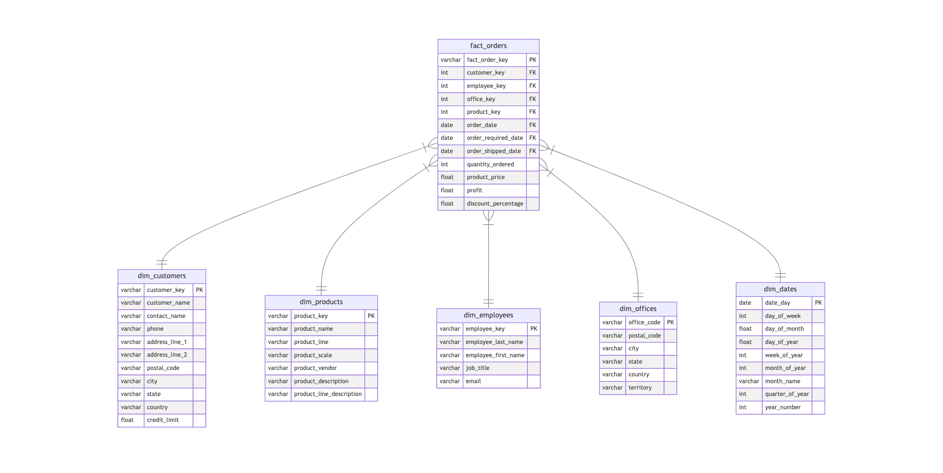
4.2 - Star Schema

Here is the new ERM diagram for the star schema, which was modified to include some transformations. You will use Spark SQL to bring the necessary columns for each table. Then you will perform additional operations to the resulting dataframe and store the resulting data in the classicmodels_star_schema schema in the Postgres RDS.

4.3 - Customers Dimension

Let’s start with the dimensional tables, first with the customers dimension.

4.3.1. Create a SQL query that brings the relevant columns from the customers temporal view and stores the query result in a Spark dataframe. Follow the instructions to prepare the query:

You need to create a column customer_number based on the customerNumber, which will be a surrogate key customer_key later. This function requires an array of text columns so you will need to cast() the customerNumber to string.
For this new data model you are required to create the field contact_name which is a combination of the contactFirstName and contactLastName fields. You can use the function concat().

select_query_customers = """
SELECT 
    cast(customerNumber as string) as customer_number, 
    customerName as customer_name,
    concat(contactFirstName, contactLastName) as contact_name, 
    phone as phone, 
    addressLine1 as address_line_1, 
    addressLine2 as address_line_2, 
    postalCode as postal_code, 
    city as city, 
    state as state, 
    country as country,
    creditLimit as credit_limit
FROM customers
"""

dim_customers_df = spark.sql(select_query_customers)

VBox()

FloatProgress(value=0.0, bar_style='info', description='Progress:', layout=Layout(height='25px', width='50%'),…

4.3.2. Now, with the resulting dim_customers_df dataframe:

Call the surrogateUDF to generate a surrogate key based on the customer_number. You will need to use array() function to convert it to an array.
Add the surrogate key using the withColumn() function, call the new column customer_key.

Then perform a select to grab the columns related to the ERM diagram.

dim_customers_df = dim_customers_df.withColumn("customer_key", surrogateUDF(array("customer_number")))\
.select(["customer_key","customer_name","contact_name","phone","address_line_1","address_line_2","postal_code","city","state","country","credit_limit"])

VBox()

FloatProgress(value=0.0, bar_style='info', description='Progress:', layout=Layout(height='25px', width='50%'),…

4.3.3. Now, store the final dataframe into the classicmodels_star_schema schema, creating a new table called dim_customers.

dim_customers_df.write.jdbc(url=jdbc_url, table="classicmodels_star_schema.dim_customers", mode="overwrite", properties=jdbc_properties)

VBox()

FloatProgress(value=0.0, bar_style='info', description='Progress:', layout=Layout(height='25px', width='50%'),…

4.3.4. Check that the table is stored in the schema:

dim_customers_df_check = spark.read.jdbc(url=jdbc_url, table="classicmodels_star_schema.dim_customers", properties=jdbc_properties)

print("dim_customers column names: ", dim_customers_df_check.columns)

dim_customers_row_count = dim_customers_df_check.count()
print("dim_customers number of rows: ", dim_customers_row_count)

VBox()

FloatProgress(value=0.0, bar_style='info', description='Progress:', layout=Layout(height='25px', width='50%'),…

dim_customers column names:  ['customer_key', 'customer_name', 'contact_name', 'phone', 'address_line_1', 'address_line_2', 'postal_code', 'city', 'state', 'country', 'credit_limit']
dim_customers number of rows:  122

Expected Output

dim_customers column names:  ['customer_key', 'customer_name', 'contact_name', 'phone', 'address_line_1', 'address_line_2', 'postal_code', 'city', 'state', 'country', 'credit_limit']
dim_customers number of rows:  122

4.4 - Products Dimension

Continue with the products dimension.

4.4.1. Create a SQL query that brings the relevant columns from the products temporal view and stores the query result in a Spark dataframe. Later you will create a surrogate key product_key based on the productCode. The productCode is already a string, so you don’t have to cast it - just select it for now and name as product_code for consistency.

select_query_products = """
SELECT 
    productCode as product_code, 
    productName as product_name, 
    products.productLine as product_line, 
    productScale as product_scale, 
    productVendor as product_vendor,
    productDescription as product_description, 
    textDescription as product_line_description
FROM products
JOIN productlines ON products.productLine=productlines.productLine
"""

dim_products_df = spark.sql(select_query_products)

VBox()

FloatProgress(value=0.0, bar_style='info', description='Progress:', layout=Layout(height='25px', width='50%'),…

4.4.2. With the resulting dim_products_df dataframe:

Call the surrogateUDF to generate a surrogate key based on the product_code. You will need to use array() function to convert it to an array.
Add the surrogate key using the withColumn() function, call the new column product_key.

Then perform a select to grab the columns related to the ERM diagram.

dim_products_df = dim_products_df.withColumn("product_key", surrogateUDF(array("product_code")))\
.select(["product_key","product_name","product_line","product_scale","product_vendor","product_description","product_line_description"])

VBox()

FloatProgress(value=0.0, bar_style='info', description='Progress:', layout=Layout(height='25px', width='50%'),…

4.4.3. Store the dim_products_df dataframe into the classicmodels_star_schema schema, table dim_products (see how it was done in the step 4.3.3).

dim_products_df.write.jdbc(url=jdbc_url, table="classicmodels_star_schema.dim_products", mode="overwrite", properties=jdbc_properties)

VBox()

FloatProgress(value=0.0, bar_style='info', description='Progress:', layout=Layout(height='25px', width='50%'),…

4.4.4. Check your work:

dim_products_df_check = spark.read.jdbc(url=jdbc_url, table="classicmodels_star_schema.dim_products", properties=jdbc_properties)

print("dim_products column names: ", dim_products_df_check.columns)

dim_products_row_count = dim_products_df_check.count()
print("dim_products number of rows: ", dim_products_row_count)

VBox()

FloatProgress(value=0.0, bar_style='info', description='Progress:', layout=Layout(height='25px', width='50%'),…

dim_products column names:  ['product_key', 'product_name', 'product_line', 'product_scale', 'product_vendor', 'product_description', 'product_line_description']
dim_products number of rows:  110

Expected Output

dim_products column names:  ['product_key', 'product_name', 'product_line', 'product_scale', 'product_vendor', 'product_description', 'product_line_description']
dim_products number of rows:  110

4.5 - Offices Dimension

Now, let’s proceed with the offices dimension.

4.5.1. Create a SQL query that brings the relevant columns from the offices temporal table and stores the query result in a Spark dataframe. Later you will create a surrogate key office_key based on the officeCode. The officeCode is already a string, so you don’t have to cast it - just select it for now and name as office_code for consistency.

select_query_offices = """
SELECT 
    officeCode as office_code, 
    postalCode as postal_code, 
    city as city, 
    state as state, 
    country as country, 
    territory as territory
FROM offices
"""

dim_offices_df = spark.sql(select_query_offices)

VBox()

FloatProgress(value=0.0, bar_style='info', description='Progress:', layout=Layout(height='25px', width='50%'),…

4.5.2. With the resulting dim_offices_df dataframe:

Call the surrogateUDF to generate a surrogate key based on the office_code. You will need to use array() function to convert it to an array.
Add the surrogate key using the withColumn() function, call the new column office_key.

Then perform a select to grab the columns related to the ERM diagram.

dim_offices_df = dim_offices_df.withColumn("office_key", surrogateUDF(array("office_code")))\
.select(["office_key","postal_code","city","state","country","territory"])

VBox()

FloatProgress(value=0.0, bar_style='info', description='Progress:', layout=Layout(height='25px', width='50%'),…

4.5.3. Store the dim_offices_df dataframe into the classicmodels_star_schema schema, table dim_offices.

dim_offices_df.write.jdbc(url=jdbc_url, table="classicmodels_star_schema.dim_offices", mode="overwrite", properties=jdbc_properties)

VBox()

FloatProgress(value=0.0, bar_style='info', description='Progress:', layout=Layout(height='25px', width='50%'),…

4.5.4. Check your work:

dim_offices_df_check = spark.read.jdbc(url=jdbc_url, table="classicmodels_star_schema.dim_offices", properties=jdbc_properties)

print("dim_offices column names: ", dim_offices_df_check.columns)

dim_offices_row_count = dim_offices_df_check.count()
print("dim_offices number of rows: ", dim_offices_row_count)

VBox()

FloatProgress(value=0.0, bar_style='info', description='Progress:', layout=Layout(height='25px', width='50%'),…

dim_offices column names:  ['office_key', 'postal_code', 'city', 'state', 'country', 'territory']
dim_offices number of rows:  7

Expected Output

dim_offices column names:  ['office_key', 'postal_code', 'city', 'state', 'country', 'territory']
dim_offices number of rows:  7

4.6 - Employees Dimension

Let’s continue with the employees dimension.

4.6.1. Follow similar steps to create employees dimension. There will be a surrogate key employee_key based on the employeeNumber. You’ll need to create a column employee_number based on the employeeNumber. Cast to string with the function cast().

select_query_employees = """
SELECT 
    cast(employeeNumber as string) as employee_number,
    lastName as employee_last_name, 
    firstName as employee_first_name, 
    jobTitle as job_title, 
    email as email
FROM employees
"""

dim_employees_df = spark.sql(select_query_employees)

VBox()

FloatProgress(value=0.0, bar_style='info', description='Progress:', layout=Layout(height='25px', width='50%'),…

4.6.2. With the resulting dim_employees_df dataframe:

Call the surrogateUDF to generate a surrogate key based on the employee_number. You will need to use array() function to convert it to an array.
Add the surrogate key using the withColumn() function, call the new column employee_key.

Then perform a select to grab the columns related to the ERM diagram.

dim_employees_df = dim_employees_df.withColumn("employee_key", surrogateUDF(array("employee_number")))\
.select(["employee_key","employee_last_name","employee_first_name","email"])

VBox()

FloatProgress(value=0.0, bar_style='info', description='Progress:', layout=Layout(height='25px', width='50%'),…

4.6.3. Store the dim_employees_df dataframe into the classicmodels_star_schema schema, table dim_employees.

dim_employees_df.write.jdbc(url=jdbc_url, table="classicmodels_star_schema.dim_employees", mode="overwrite", properties=jdbc_properties)

VBox()

FloatProgress(value=0.0, bar_style='info', description='Progress:', layout=Layout(height='25px', width='50%'),…

4.6.4. Check your work:

dim_employees_df_check = spark.read.jdbc(url=jdbc_url, table="classicmodels_star_schema.dim_employees", properties=jdbc_properties)

print("dim_employees column names: ", dim_employees_df_check.columns)

dim_employees_row_count = dim_employees_df_check.count()
print("dim_employees number of rows: ", dim_employees_row_count)

VBox()

FloatProgress(value=0.0, bar_style='info', description='Progress:', layout=Layout(height='25px', width='50%'),…

dim_employees column names:  ['employee_key', 'employee_last_name', 'employee_first_name', 'email']
dim_employees number of rows:  23

Expected Output

dim_employees column names:  ['employee_key', 'employee_last_name', 'employee_first_name', 'email']
dim_employees number of rows:  23

4.7 - Date Dimension

4.7.1. As in the dbt lab, you will limit the date’s dimension table to the dates that appear in the orders table. You are already provided with the date range required to create your dimension table. In the following cell, you will:

Use the to_date function to enclose the start_date and end_date strings to convert them into actual date types.
Use the sequence function from psypark.sql.functions to generate a sequence of values from the start_date to the end_date. Note that the third parameter is the interval, which has been set to interval 1 day. The result from the sequence function is an array of values.
Finally, enclose the sequence function into the explode function. This function takes an array and returns one row for each element in the array. Note how the column has been named date_day.

from pyspark.sql.functions import col, explode, sequence, year, month, dayofweek, dayofmonth, dayofyear, weekofyear, date_format, lit
from pyspark.sql.types import DateType

# Date range
start_date = "2003-01-01"
end_date = "2005-12-31"

date_range_df = spark.sql(f"SELECT explode(sequence(to_date('{start_date}'), to_date('{end_date}'), interval 1 day)) as date_day")

VBox()

FloatProgress(value=0.0, bar_style='info', description='Progress:', layout=Layout(height='25px', width='50%'),…

4.7.2. Based on the date_range_df dataframe, you are going to create the following columns by using the withColumn():

Get the day of the week with the dayofweek() function; store it at the column day_of_week.
Get the day of the month with the dayofmonth() function; store it at the column day_of_month.
Get the number of the day in the year with the dayofyear() function; store it in the column day_of_year.
Get the number of the week in the year with the weekofyear() function; store it in the column week_of_year.
Get the the month with the month() function; store it at the column month_of_year.
Get the the year with the year() function; store it at the column year_number.

Also, you will be creating a column month_name, but the code is already complete for that.

In addition, you are going to create the quarter_of_year column by creating a new UDF. This time, instead of using the UDF as an SQL function with SparkSQL, you will register it as a Python UDF.

Complete the get_quarter_of_year() function by making an integer division between date.month - 1 and 3 (with the // operator). Then, add 1 and return the value.
Call the udf() function and pass it as parameters to the function you just created and the IntegerType() function.

def get_quarter_of_year(date):
    return (date.month - 1) // 3 + 1

get_quarter_of_year_udf = udf(get_quarter_of_year, IntegerType())

VBox()

FloatProgress(value=0.0, bar_style='info', description='Progress:', layout=Layout(height='25px', width='50%'),…

date_dim_df = date_range_df.withColumn("day_of_week", dayofweek("date_day")) \
    .withColumn("day_of_month", dayofmonth("date_day")) \
    .withColumn("day_of_year", dayofyear("date_day")) \
    .withColumn("week_of_year", weekofyear("date_day")) \
    .withColumn("month_of_year", month("date_day")) \
    .withColumn("year_number", year("date_day")) \
    .withColumn("month_name", date_format("date_day", "MMMM")) \
    .withColumn("quarter_of_year", get_quarter_of_year_udf("date_day"))

# Show the result
date_dim_df.show()

VBox()



FloatProgress(value=0.0, bar_style='info', description='Progress:', layout=Layout(height='25px', width='50%'),…


+----------+-----------+------------+-----------+------------+-------------+-----------+----------+---------------+
|  date_day|day_of_week|day_of_month|day_of_year|week_of_year|month_of_year|year_number|month_name|quarter_of_year|
+----------+-----------+------------+-----------+------------+-------------+-----------+----------+---------------+
|2003-01-01|          4|           1|          1|           1|            1|       2003|   January|              1|
|2003-01-02|          5|           2|          2|           1|            1|       2003|   January|              1|
|2003-01-03|          6|           3|          3|           1|            1|       2003|   January|              1|
|2003-01-04|          7|           4|          4|           1|            1|       2003|   January|              1|
|2003-01-05|          1|           5|          5|           1|            1|       2003|   January|              1|
|2003-01-06|          2|           6|          6|           2|            1|       2003|   January|              1|
|2003-01-07|          3|           7|          7|           2|            1|       2003|   January|              1|
|2003-01-08|          4|           8|          8|           2|            1|       2003|   January|              1|
|2003-01-09|          5|           9|          9|           2|            1|       2003|   January|              1|
|2003-01-10|          6|          10|         10|           2|            1|       2003|   January|              1|
|2003-01-11|          7|          11|         11|           2|            1|       2003|   January|              1|
|2003-01-12|          1|          12|         12|           2|            1|       2003|   January|              1|
|2003-01-13|          2|          13|         13|           3|            1|       2003|   January|              1|
|2003-01-14|          3|          14|         14|           3|            1|       2003|   January|              1|
|2003-01-15|          4|          15|         15|           3|            1|       2003|   January|              1|
|2003-01-16|          5|          16|         16|           3|            1|       2003|   January|              1|
|2003-01-17|          6|          17|         17|           3|            1|       2003|   January|              1|
|2003-01-18|          7|          18|         18|           3|            1|       2003|   January|              1|
|2003-01-19|          1|          19|         19|           3|            1|       2003|   January|              1|
|2003-01-20|          2|          20|         20|           4|            1|       2003|   January|              1|
+----------+-----------+------------+-----------+------------+-------------+-----------+----------+---------------+
only showing top 20 rows

4.7.3. Store the date_dim_df dataframe into the classicmodels_star_schema schema, table dim_date.

date_dim_df.write.jdbc(url=jdbc_url, table="classicmodels_star_schema.dim_date", mode="overwrite", properties=jdbc_properties)

VBox()

FloatProgress(value=0.0, bar_style='info', description='Progress:', layout=Layout(height='25px', width='50%'),…

4.7.4. Check that your table was correctly stored in the schema:

date_dim_df_check = spark.read.jdbc(url=jdbc_url, table="classicmodels_star_schema.dim_date", properties=jdbc_properties)

print("dim_date column names: ", date_dim_df_check.columns)

dim_employees_row_count = date_dim_df_check.count()
print("dim_date number of rows: ", dim_employees_row_count)

VBox()

FloatProgress(value=0.0, bar_style='info', description='Progress:', layout=Layout(height='25px', width='50%'),…

dim_date column names:  ['date_day', 'day_of_week', 'day_of_month', 'day_of_year', 'week_of_year', 'month_of_year', 'year_number', 'month_name', 'quarter_of_year']
dim_date number of rows:  1096

Expected Output

dim_date column names:  ['date_day', 'day_of_week', 'day_of_month', 'day_of_year', 'week_of_year', 'month_of_year', 'year_number', 'month_name', 'quarter_of_year']
dim_date number of rows:  1096

4.8 - Fact Table

Finally, let’s create the orders fact table. Remember that the fact table stores the surrogate keys to the dimensional tables and the numerical facts related to the business process.

There has been a change in the model compared to the Week 1 assignment. You will add two new facts:

profit: metric calculated by subtracting the price of the product as we sell by the price we bought the product at.
discount_percentage: metric calculated by subtracting the MSRP of a product from the selling price, dividing the result by the same MSRP and then multiplying the result by 100.

4.8.1. Here is the statement to bring all the relevant columns and create the data model into the fact_table_df dataframe. There are also corresponding operations to add the missing calculated columns.

select_query_fact = """
SELECT 
    orders.orderNumber, 
    cast(orderdetails.orderLineNumber as string) as order_line_number,
    cast(orders.customerNumber as string) as customer_number, 
    cast(employees.employeeNumber as string) as employee_number,
    offices.officeCode,
    orderdetails.productCode, 
    orders.orderDate as order_date,
    orders.requiredDate as order_required_date, 
    orders.shippedDate as order_shipped_date,
    orderdetails.quantityOrdered as quantity_ordered, 
    orderdetails.priceEach as product_price,
    (orderdetails.priceEach - products.buyPrice) as profit,
    (products.msrp - orderdetails.priceEach)/products.msrp * 100 as discount_percentage
FROM orders
JOIN orderdetails ON orders.orderNumber = orderdetails.orderNumber
JOIN customers ON orders.customerNumber = customers.customerNumber
JOIN employees ON customers.salesRepEmployeeNumber = employees.employeeNumber
JOIN offices ON employees.officeCode = offices.officeCode
JOIN products ON products.productCode = orderdetails.productCode
""";

fact_table_df = spark.sql(select_query_fact)

VBox()

FloatProgress(value=0.0, bar_style='info', description='Progress:', layout=Layout(height='25px', width='50%'),…

4.8.2. Add the calculated facts and the required surrogate keys. Use function surrogateUDF() passing an array based on:

customer_number for the customer_key,
employee_number for the employee_key,
officeCode for the office_key,
productCode for the product_key.

fact_table_df = fact_table_df.withColumn("fact_order_key", surrogateUDF(array("orderNumber", "order_line_number")))\
.withColumn("customer_key", surrogateUDF(array("customer_number")))\
.withColumn("employee_key", surrogateUDF(array("employee_number")))\
.withColumn("office_key", surrogateUDF(array("officeCode")))\
.withColumn("product_key", surrogateUDF(array("productCode")))\
.select(["fact_order_key","customer_key","employee_key","office_key","product_key","order_date","order_required_date","order_shipped_date","quantity_ordered","product_price","profit","discount_percentage"])

VBox()

FloatProgress(value=0.0, bar_style='info', description='Progress:', layout=Layout(height='25px', width='50%'),…

4.8.3. Store the result in the fact_orders table in your database classicmodels_star_schema.

fact_table_df.write.jdbc(url=jdbc_url, table="classicmodels_star_schema.fact_orders", mode="overwrite", properties=jdbc_properties)

VBox()

FloatProgress(value=0.0, bar_style='info', description='Progress:', layout=Layout(height='25px', width='50%'),…

4.8.4. Check that your table was correctly stored in the schema:

fact_table_df_check = spark.read.jdbc(url=jdbc_url, table="classicmodels_star_schema.fact_orders", properties=jdbc_properties)

print("fact_orders column names: ", fact_table_df_check.columns)

fact_table_row_count = fact_table_df_check.count()
print("fact_orders number of rows: ", fact_table_row_count)

VBox()

FloatProgress(value=0.0, bar_style='info', description='Progress:', layout=Layout(height='25px', width='50%'),…

fact_orders column names:  ['fact_order_key', 'customer_key', 'employee_key', 'office_key', 'product_key', 'order_date', 'order_required_date', 'order_shipped_date', 'quantity_ordered', 'product_price', 'profit', 'discount_percentage']
fact_orders number of rows:  2996

Expected Output

fact_orders column names:  ['fact_order_key', 'customer_key', 'employee_key', 'office_key', 'product_key', 'order_date', 'order_required_date', 'order_shipped_date', 'quantity_ordered', 'product_price', 'profit', 'discount_percentage']
fact_orders number of rows:  2996

4.8.5. Finally, print out your schema:

fact_table_df.printSchema()

VBox()



FloatProgress(value=0.0, bar_style='info', description='Progress:', layout=Layout(height='25px', width='50%'),…


root
 |-- fact_order_key: string (nullable = true)
 |-- customer_key: string (nullable = true)
 |-- employee_key: string (nullable = true)
 |-- office_key: string (nullable = true)
 |-- product_key: string (nullable = true)
 |-- order_date: timestamp (nullable = true)
 |-- order_required_date: timestamp (nullable = true)
 |-- order_shipped_date: timestamp (nullable = true)
 |-- quantity_ordered: integer (nullable = true)
 |-- product_price: decimal(38,18) (nullable = true)
 |-- profit: decimal(38,17) (nullable = true)
 |-- discount_percentage: decimal(38,6) (nullable = true)

Expected Output

root
 |-- fact_order_key: string (nullable = true)
 |-- customer_key: string (nullable = true)
 |-- employee_key: string (nullable = true)
 |-- office_key: string (nullable = true)
 |-- product_key: string (nullable = true)
 |-- order_date: timestamp (nullable = true)
 |-- order_required_date: timestamp (nullable = true)
 |-- order_shipped_date: timestamp (nullable = true)
 |-- quantity_ordered: integer (nullable = true)
 |-- product_price: decimal(38,18) (nullable = true)
 |-- profit: decimal(38,17) (nullable = true)
 |-- discount_percentage: decimal(38,6) (nullable = true)

In this lab, you have explored basic data transformation using Apache Spark, focusing on the capabilities of their Python API (PySpark) and Spark SQL. These tools are essential for data engineers, offering powerful and efficient methods for manipulating large datasets. Spark offers rich APIs and tools for data transformations, one of them being Spark SQL, which enables querying of structured data with SQL-like syntax. Although this dataset isn’t particularly large, the same principles apply to larger data sources due to data parallelism.

5 - Upload Files for Grading

Upload the notebook into S3 bucket for grading purposes.

Note: you may need to click Save button before the upload.

In your AWS console, search again for CloudShell and click on it. Once the terminal is ready, execute the following two commands to upload your notebook:

export ACCOUNT_ID=$(aws sts get-caller-identity --query Account --output text)

aws s3 cp s3://de-c4w3a1-$ACCOUNT_ID-us-east-1-emr-bucket/emr-studio/$(aws s3 ls s3://de-c4w3a1-$ACCOUNT_ID-us-east-1-emr-bucket/emr-studio --recursive | grep -o "e-[^/]*" | head -n 1)/C4_W3_Assignment.ipynb s3://de-c4w3a1-$ACCOUNT_ID-us-east-1-submission/C4_W3_Assignment_Learner.ipynb

coursera-data-engineering

Data Transformations with Apache Spark

Table of Contents

1 - Introduction

2 - Environment Setup

3 - Apache Spark 101

3.1 - Spark Classes

3.2 - Spark Dataframe

3.3 - Spark SQL

3.4 - UDFs and Data Types

4 - Data Modeling with Spark

4.1 - Read the Tables

4.2 - Star Schema

4.3 - Customers Dimension

Expected Output

4.4 - Products Dimension

Expected Output

4.5 - Offices Dimension

Expected Output

4.6 - Employees Dimension

Expected Output

4.7 - Date Dimension

Expected Output

4.8 - Fact Table

Expected Output

Expected Output

5 - Upload Files for Grading