coursera-data-engineering
Week 4 Lab: Data Visualization with DBT and Superset
During this week’s lab, you will learn how to create analytical views and a dashboard.
Table of Contents
Load the SQL extension.
%load_ext sql
1 - Introduction and Setup
Data visualization is a critical skill for a Data Engineer, enabling you to transform complex data sets into insightful, actionable visuals. Effective visual communication can enhance understanding of the insights you gained while processing data, uncover trends, and drive strategic actions in any data-centric organization. In this lab, you will use a star schema model created on top of the classicmodels dataset, you will create analytical views on top of this model and then display the results in a dashboard using Apache Superset.
dbt is a transformation workflow command line tool based on SQL, you have worked with dbt before and the initial project is similar to the one done for the assignment of the first week of this course.
Let’s start the dbt project called classicmodels_modeling.
Note: All terminal commands in this lab should be run in the VSCode terminal, not Jupyter, as it may cause some issues. Always check that the virtual environment is active.
1.1.1. Activate the Python virtual environment for the lab. Run the following command in the VSCode terminal:
source jupyterlab-venv/bin/activate
1.1.2. Check that dbt Core is installed.
dbt --version
1.1.3. Go to AWS console, and in the CloudFormation Outputs tab find the key PostgresEndpoint. Copy the corresponding Value.
1.1.4. Open the file located at ./scripts/profiles.yml. Replace the placeholders <DATABASE_ENDPOINT> with the endpoint value. Save changes.
1.1.5. Run the following command to copy the profiles.yml file to the invisible folder .dbt of the project:
cp ./scripts/profiles.yml $HOME/.dbt/profiles.yml
1.1.6. Navigate into your project’s directory:
cd classicmodels_modeling
1.1.7. Run the following command to test the connection:
dbt debug
It should return a Connection test: OK connection ok at the end of the output.
1.1.8. Run the following command to fetch the latest stable versions of tools and libraries specified in the packages.yml file.
dbt deps
1.1.9. Load the source configuration into the notebook with the following code:
import yaml

with open("./scripts/profiles.yml", 'r') as stream:
    data_loaded = yaml.safe_load(stream)

DBCONFIG = data_loaded["classicmodels_modeling"]["outputs"]["source"]
DBHOST = DBCONFIG["host"]
DBPORT = int(DBCONFIG["port"])
DBNAME = DBCONFIG["dbname"]
DBUSER = DBCONFIG["user"]
DBPASSWORD = DBCONFIG["password"]
db_connection_url = f'postgresql+psycopg2://{DBUSER}:{DBPASSWORD}@{DBHOST}:{DBPORT}/{DBNAME}'

%sql {db_connection_url}
1.1.10. Test the connection from the Notebook to the Postgres database. You should see the schemas of the database in the output.
%%sql

SELECT schema_name
FROM information_schema.schemata;
 * postgresql+psycopg2://postgresuser:***@de-c4w4lab1-rds.cd044wq8gkrk.us-east-1.rds.amazonaws.com:5432/postgres
4 rows affected.
| schema_name |
|---|
| public |
| classicmodels |
| information_schema |
| pg_catalog |
1.1.11. Run the star schema models in the VSCode terminal (make sure that you are still in the project directory classicmodels_modeling):
dbt run
You should see a similar output to the run command:
Finished running 7 table models in 0 hours 0 minutes and 1.xx seconds (1.xx s).

Completed successfully

Done. PASS=7 WARN=0 ERROR=0 SKIP=0 TOTAL=7
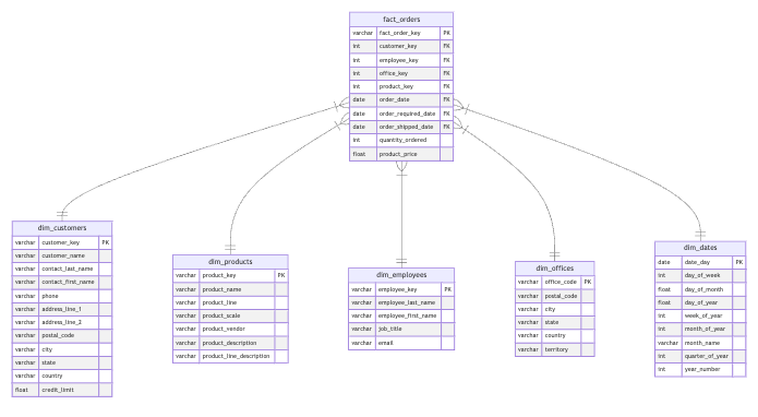
1.1.12. Verify that the star schema was added to the Postgres database, the new schema should be called classicmodels_star_schema:
%%sql

SELECT schema_name
FROM information_schema.schemata;
 * postgresql+psycopg2://postgresuser:***@de-c4w4lab1-rds.cd044wq8gkrk.us-east-1.rds.amazonaws.com:5432/postgres
5 rows affected.
| schema_name |
|---|
| public |
| classicmodels_star_schema |
| classicmodels |
| information_schema |
| pg_catalog |
1.1.13. Now, let’s verify that the star schema fact and dimensional tables are available in the new schema. Run the following cell:
%%sql
SELECT table_catalog, table_schema, table_name, table_type  FROM information_schema.tables
WHERE table_schema = 'classicmodels_star_schema'
 * postgresql+psycopg2://postgresuser:***@de-c4w4lab1-rds.cd044wq8gkrk.us-east-1.rds.amazonaws.com:5432/postgres
7 rows affected.
| table_catalog | table_schema | table_name | table_type |
|---|---|---|---|
| postgres | classicmodels_star_schema | dim_dates | BASE TABLE |
| postgres | classicmodels_star_schema | dates | BASE TABLE |
| postgres | classicmodels_star_schema | dim_customers | BASE TABLE |
| postgres | classicmodels_star_schema | dim_employees | BASE TABLE |
| postgres | classicmodels_star_schema | dim_offices | BASE TABLE |
| postgres | classicmodels_star_schema | dim_products | BASE TABLE |
| postgres | classicmodels_star_schema | fact_orders | BASE TABLE |
Verify that each table has data and their columns names and types.
%sql SELECT * FROM classicmodels_star_schema.fact_orders LIMIT 10
 * postgresql+psycopg2://postgresuser:***@de-c4w4lab1-rds.cd044wq8gkrk.us-east-1.rds.amazonaws.com:5432/postgres
10 rows affected.
| fact_order_key | customer_key | employee_key | office_key | product_key | order_date | order_required_date | order_shipped_date | quantity_ordered | product_price |
|---|---|---|---|---|---|---|---|---|---|
| 1f8f31c7d43a69e00bff8264109eeb4c | 00411460f7c92d2124a67ea0f4cb5f85 | 3948ead63a9f2944218de038d8934305 | c81e728d9d4c2f636f067f89cc14862c | f95ed59fd3313855e03af1b96334e685 | 2003-01-06 00:00:00 | 2003-01-13 00:00:00 | 2003-01-10 00:00:00 | 30 | 136 |
| 98242fbce3c533a4ae5827f13142af23 | 00411460f7c92d2124a67ea0f4cb5f85 | 3948ead63a9f2944218de038d8934305 | c81e728d9d4c2f636f067f89cc14862c | e99d5f4747d9abb3e4148d0317dac3df | 2003-01-06 00:00:00 | 2003-01-13 00:00:00 | 2003-01-10 00:00:00 | 50 | 55.09 |
| 3b73bc66e4119eacbc3c63eaf4608548 | 00411460f7c92d2124a67ea0f4cb5f85 | 3948ead63a9f2944218de038d8934305 | c81e728d9d4c2f636f067f89cc14862c | 429d1bfa2660c76daf6d27f99e10c40e | 2003-01-06 00:00:00 | 2003-01-13 00:00:00 | 2003-01-10 00:00:00 | 22 | 75.46 |
| 969259c8f1be79a73de9014d18c56827 | 00411460f7c92d2124a67ea0f4cb5f85 | 3948ead63a9f2944218de038d8934305 | c81e728d9d4c2f636f067f89cc14862c | 62b141855439f4ba3f52036409a9fd14 | 2003-01-06 00:00:00 | 2003-01-13 00:00:00 | 2003-01-10 00:00:00 | 49 | 35.29 |
| 85fc329e6a3e29d44ae81fd0f0809edf | 76dc611d6ebaafc66cc0879c71b5db5c | 49b8b4f95f02e055801da3b4f58e28b7 | 8f14e45fceea167a5a36dedd4bea2543 | ef8e0274836db61155b2f6329206ffb6 | 2003-01-09 00:00:00 | 2003-01-18 00:00:00 | 2003-01-11 00:00:00 | 25 | 108.06 |
| ba8b8ce928e516b27b249b7ab87d7eb7 | 76dc611d6ebaafc66cc0879c71b5db5c | 49b8b4f95f02e055801da3b4f58e28b7 | 8f14e45fceea167a5a36dedd4bea2543 | 9bdf7d6aaeffea97a4ab0f562fe54026 | 2003-01-09 00:00:00 | 2003-01-18 00:00:00 | 2003-01-11 00:00:00 | 26 | 167.06 |
| 18d5bb62b3a7d1e610f32b0b06f5c900 | 76dc611d6ebaafc66cc0879c71b5db5c | 49b8b4f95f02e055801da3b4f58e28b7 | 8f14e45fceea167a5a36dedd4bea2543 | 7e1421596451e8efe4ac99cf6fc783be | 2003-01-09 00:00:00 | 2003-01-18 00:00:00 | 2003-01-11 00:00:00 | 45 | 32.53 |
| 8272d88bcb8ca0786f887b9b31e903a6 | 76dc611d6ebaafc66cc0879c71b5db5c | 49b8b4f95f02e055801da3b4f58e28b7 | 8f14e45fceea167a5a36dedd4bea2543 | fb74c462a79ab6342c1a81bfb0bbd8d8 | 2003-01-09 00:00:00 | 2003-01-18 00:00:00 | 2003-01-11 00:00:00 | 46 | 44.35 |
| c5ee31aea3ebb5f4e85821ac18f1ab2d | fc221309746013ac554571fbd180e1c8 | c0a271bc0ecb776a094786474322cb82 | eccbc87e4b5ce2fe28308fd9f2a7baf3 | 2f1940aaee16632276d6ba6b5b709615 | 2003-01-10 00:00:00 | 2003-01-18 00:00:00 | 2003-01-14 00:00:00 | 39 | 95.55 |
| 47a313d1eb63620f42d485ac2e4da78d | fc221309746013ac554571fbd180e1c8 | c0a271bc0ecb776a094786474322cb82 | eccbc87e4b5ce2fe28308fd9f2a7baf3 | cd0f60c4410a9de77da04fb01e74c504 | 2003-01-10 00:00:00 | 2003-01-18 00:00:00 | 2003-01-14 00:00:00 | 41 | 43.13 |
%sql SELECT * FROM classicmodels_star_schema.dim_customers LIMIT 10
 * postgresql+psycopg2://postgresuser:***@de-c4w4lab1-rds.cd044wq8gkrk.us-east-1.rds.amazonaws.com:5432/postgres
10 rows affected.
| customer_key | customer_name | customer_last_name | customer_first_name | phone | address_line_1 | address_line_2 | postal_code | city | state | country | creditlimit |
|---|---|---|---|---|---|---|---|---|---|---|---|
| 6974ce5ac660610b44d9b9fed0ff9548 | Atelier graphique | Schmitt | Carine | 40.32.2555 | 54, rue Royale | None | 44000 | Nantes | None | France | 21000 |
| 7f6ffaa6bb0b408017b62254211691b5 | Signal Gift Stores | King | Jean | 7025551838 | 8489 Strong St. | None | 83030 | Las Vegas | NV | USA | 71800 |
| 5fd0b37cd7dbbb00f97ba6ce92bf5add | Australian Collectors, Co. | Ferguson | Peter | 03 9520 4555 | 636 St Kilda Road | Level 3 | 3004 | Melbourne | Victoria | Australia | 117300 |
| 07e1cd7dca89a1678042477183b7ac3f | La Rochelle Gifts | Labrune | Janine | 40.67.8555 | 67, rue des Cinquante Otages | None | 44000 | Nantes | None | France | 118200 |
| 4c56ff4ce4aaf9573aa5dff913df997a | Baane Mini Imports | Bergulfsen | Jonas | 07-98 9555 | Erling Skakkes gate 78 | None | 4110 | Stavern | None | Norway | 81700 |
| c8ffe9a587b126f152ed3d89a146b445 | Mini Gifts Distributors Ltd. | Nelson | Susan | 4155551450 | 5677 Strong St. | None | 97562 | San Rafael | CA | USA | 210500 |
| 3def184ad8f4755ff269862ea77393dd | Havel & Zbyszek Co | Piestrzeniewicz | Zbyszek | (26) 642-7555 | ul. Filtrowa 68 | None | 01-012 | Warszawa | None | Poland | 0 |
| 76dc611d6ebaafc66cc0879c71b5db5c | Blauer See Auto, Co. | Keitel | Roland | +49 69 66 90 2555 | Lyonerstr. 34 | None | 60528 | Frankfurt | None | Germany | 59700 |
| d1f491a404d6854880943e5c3cd9ca25 | Mini Wheels Co. | Murphy | Julie | 6505555787 | 5557 North Pendale Street | None | 94217 | San Francisco | CA | USA | 64600 |
| 1afa34a7f984eeabdbb0a7d494132ee5 | Land of Toys Inc. | Lee | Kwai | 2125557818 | 897 Long Airport Avenue | None | 10022 | NYC | NY | USA | 114900 |
%sql SELECT * FROM classicmodels_star_schema.dim_employees LIMIT 10
 * postgresql+psycopg2://postgresuser:***@de-c4w4lab1-rds.cd044wq8gkrk.us-east-1.rds.amazonaws.com:5432/postgres
10 rows affected.
| employee_key | employee_last_name | employee_first_name | job_title | |
|---|---|---|---|---|
| fba9d88164f3e2d9109ee770223212a0 | Murphy | Diane | President | dmurphy@classicmodelcars.com |
| 4ca82782c5372a547c104929f03fe7a9 | Patterson | Mary | VP Sales | mpatterso@classicmodelcars.com |
| 8a1e808b55fde9455cb3d8857ed88389 | Firrelli | Jeff | VP Marketing | jfirrelli@classicmodelcars.com |
| b1563a78ec59337587f6ab6397699afc | Patterson | William | Sales Manager (APAC) | wpatterson@classicmodelcars.com |
| c667d53acd899a97a85de0c201ba99be | Bondur | Gerard | Sale Manager (EMEA) | gbondur@classicmodelcars.com |
| 208e43f0e45c4c78cafadb83d2888cb6 | Bow | Anthony | Sales Manager (NA) | abow@classicmodelcars.com |
| a3fb4fbf9a6f9cf09166aa9c20cbc1ad | Jennings | Leslie | Sales Rep | ljennings@classicmodelcars.com |
| 0f2c9a93eea6f38fabb3acb1c31488c6 | Thompson | Leslie | Sales Rep | lthompson@classicmodelcars.com |
| c44e503833b64e9f27197a484f4257c0 | Firrelli | Julie | Sales Rep | jfirrelli@classicmodelcars.com |
| 3948ead63a9f2944218de038d8934305 | Patterson | Steve | Sales Rep | spatterson@classicmodelcars.com |
%sql SELECT * FROM classicmodels_star_schema.dim_offices LIMIT 10
 * postgresql+psycopg2://postgresuser:***@de-c4w4lab1-rds.cd044wq8gkrk.us-east-1.rds.amazonaws.com:5432/postgres
7 rows affected.
| office_key | postal_code | city | state | country | territory |
|---|---|---|---|---|---|
| c4ca4238a0b923820dcc509a6f75849b | 94080 | San Francisco | CA | USA | NA |
| c81e728d9d4c2f636f067f89cc14862c | 02107 | Boston | MA | USA | NA |
| eccbc87e4b5ce2fe28308fd9f2a7baf3 | 10022 | NYC | NY | USA | NA |
| a87ff679a2f3e71d9181a67b7542122c | 75017 | Paris | None | France | EMEA |
| e4da3b7fbbce2345d7772b0674a318d5 | 102-8578 | Tokyo | Chiyoda-Ku | Japan | Japan |
| 1679091c5a880faf6fb5e6087eb1b2dc | 2010 | Sydney | NSW | Australia | APAC |
| 8f14e45fceea167a5a36dedd4bea2543 | EC2N 1HN | London | None | UK | EMEA |
%sql SELECT * FROM classicmodels_star_schema.dim_products LIMIT 10
 * postgresql+psycopg2://postgresuser:***@de-c4w4lab1-rds.cd044wq8gkrk.us-east-1.rds.amazonaws.com:5432/postgres
10 rows affected.
| product_key | product_name | product_line | product_scale | product_vendor | product_description | product_line_description |
|---|---|---|---|---|---|---|
| c57855c679250d9702f2557f9f8c44df | 1969 Harley Davidson Ultimate Chopper | Motorcycles | 1:10 | Min Lin Diecast | This replica features working kickstand, front suspension, gear-shift lever, footbrake lever, drive chain, wheels and steering. All parts are particularly delicate due to their precise scale and require special care and attention. | Our motorcycles are state of the art replicas of classic as well as contemporary motorcycle legends such as Harley Davidson, Ducati and Vespa. Models contain stunning details such as official logos, rotating wheels, working kickstand, front suspension, gear-shift lever, footbrake lever, and drive chain. Materials used include diecast and plastic. The models range in size from 1:10 to 1:50 scale and include numerous limited edition and several out-of-production vehicles. All models come fully assembled and ready for display in the home or office. Most include a certificate of authenticity. |
| 0a113318bee26a2722998d59eaabd280 | 1952 Alpine Renault 1300 | Classic Cars | 1:10 | Classic Metal Creations | Turnable front wheels; steering function; detailed interior; detailed engine; opening hood; opening trunk; opening doors; and detailed chassis. | Attention car enthusiasts: Make your wildest car ownership dreams come true. Whether you are looking for classic muscle cars, dream sports cars or movie-inspired miniatures, you will find great choices in this category. These replicas feature superb attention to detail and craftsmanship and offer features such as working steering system, opening forward compartment, opening rear trunk with removable spare wheel, 4-wheel independent spring suspension, and so on. The models range in size from 1:10 to 1:24 scale and include numerous limited edition and several out-of-production vehicles. All models include a certificate of authenticity from their manufacturers and come fully assembled and ready for display in the home or office. |
| ff0f004a2bd95bc5437fda6accd38e4c | 1996 Moto Guzzi 1100i | Motorcycles | 1:10 | Highway 66 Mini Classics | Official Moto Guzzi logos and insignias, saddle bags located on side of motorcycle, detailed engine, working steering, working suspension, two leather seats, luggage rack, dual exhaust pipes, small saddle bag located on handle bars, two-tone paint with chrome accents, superior die-cast detail , rotating wheels , working kick stand, diecast metal with plastic parts and baked enamel finish. | Our motorcycles are state of the art replicas of classic as well as contemporary motorcycle legends such as Harley Davidson, Ducati and Vespa. Models contain stunning details such as official logos, rotating wheels, working kickstand, front suspension, gear-shift lever, footbrake lever, and drive chain. Materials used include diecast and plastic. The models range in size from 1:10 to 1:50 scale and include numerous limited edition and several out-of-production vehicles. All models come fully assembled and ready for display in the home or office. Most include a certificate of authenticity. |
| 325a76ec55097780dea7210114a8f2fd | 2003 Harley-Davidson Eagle Drag Bike | Motorcycles | 1:10 | Red Start Diecast | Model features, official Harley Davidson logos and insignias, detachable rear wheelie bar, heavy diecast metal with resin parts, authentic multi-color tampo-printed graphics, separate engine drive belts, free-turning front fork, rotating tires and rear racing slick, certificate of authenticity, detailed engine, display stand\r\n, precision diecast replica, baked enamel finish, 1:10 scale model, removable fender, seat and tank cover piece for displaying the superior detail of the v-twin engine | Our motorcycles are state of the art replicas of classic as well as contemporary motorcycle legends such as Harley Davidson, Ducati and Vespa. Models contain stunning details such as official logos, rotating wheels, working kickstand, front suspension, gear-shift lever, footbrake lever, and drive chain. Materials used include diecast and plastic. The models range in size from 1:10 to 1:50 scale and include numerous limited edition and several out-of-production vehicles. All models come fully assembled and ready for display in the home or office. Most include a certificate of authenticity. |
| 590a952a0d5589b7c925844818a4648a | 1972 Alfa Romeo GTA | Classic Cars | 1:10 | Motor City Art Classics | Features include: Turnable front wheels; steering function; detailed interior; detailed engine; opening hood; opening trunk; opening doors; and detailed chassis. | Attention car enthusiasts: Make your wildest car ownership dreams come true. Whether you are looking for classic muscle cars, dream sports cars or movie-inspired miniatures, you will find great choices in this category. These replicas feature superb attention to detail and craftsmanship and offer features such as working steering system, opening forward compartment, opening rear trunk with removable spare wheel, 4-wheel independent spring suspension, and so on. The models range in size from 1:10 to 1:24 scale and include numerous limited edition and several out-of-production vehicles. All models include a certificate of authenticity from their manufacturers and come fully assembled and ready for display in the home or office. |
| 504d67645cc129e92161e29d6f2fbd24 | 1962 LanciaA Delta 16V | Classic Cars | 1:10 | Second Gear Diecast | Features include: Turnable front wheels; steering function; detailed interior; detailed engine; opening hood; opening trunk; opening doors; and detailed chassis. | Attention car enthusiasts: Make your wildest car ownership dreams come true. Whether you are looking for classic muscle cars, dream sports cars or movie-inspired miniatures, you will find great choices in this category. These replicas feature superb attention to detail and craftsmanship and offer features such as working steering system, opening forward compartment, opening rear trunk with removable spare wheel, 4-wheel independent spring suspension, and so on. The models range in size from 1:10 to 1:24 scale and include numerous limited edition and several out-of-production vehicles. All models include a certificate of authenticity from their manufacturers and come fully assembled and ready for display in the home or office. |
| ec93374992862f071a8ade8d69da3c64 | 1968 Ford Mustang | Classic Cars | 1:12 | Autoart Studio Design | Hood, doors and trunk all open to reveal highly detailed interior features. Steering wheel actually turns the front wheels. Color dark green. | Attention car enthusiasts: Make your wildest car ownership dreams come true. Whether you are looking for classic muscle cars, dream sports cars or movie-inspired miniatures, you will find great choices in this category. These replicas feature superb attention to detail and craftsmanship and offer features such as working steering system, opening forward compartment, opening rear trunk with removable spare wheel, 4-wheel independent spring suspension, and so on. The models range in size from 1:10 to 1:24 scale and include numerous limited edition and several out-of-production vehicles. All models include a certificate of authenticity from their manufacturers and come fully assembled and ready for display in the home or office. |
| b3e8b79be1911a1f5f07d06c1a6f8d81 | 2001 Ferrari Enzo | Classic Cars | 1:12 | Second Gear Diecast | Turnable front wheels; steering function; detailed interior; detailed engine; opening hood; opening trunk; opening doors; and detailed chassis. | Attention car enthusiasts: Make your wildest car ownership dreams come true. Whether you are looking for classic muscle cars, dream sports cars or movie-inspired miniatures, you will find great choices in this category. These replicas feature superb attention to detail and craftsmanship and offer features such as working steering system, opening forward compartment, opening rear trunk with removable spare wheel, 4-wheel independent spring suspension, and so on. The models range in size from 1:10 to 1:24 scale and include numerous limited edition and several out-of-production vehicles. All models include a certificate of authenticity from their manufacturers and come fully assembled and ready for display in the home or office. |
| 3d79931afbc0f719d77cf2039dd2454b | 1958 Setra Bus | Trucks and Buses | 1:12 | Welly Diecast Productions | Model features 30 windows, skylights & glare resistant glass, working steering system, original logos | The Truck and Bus models are realistic replicas of buses and specialized trucks produced from the early 1920s to present. The models range in size from 1:12 to 1:50 scale and include numerous limited edition and several out-of-production vehicles. Materials used include tin, diecast and plastic. All models include a certificate of authenticity from their manufacturers and are a perfect ornament for the home and office. |
| a2cea97b93875997fdaf88fde1e3c2d8 | 2002 Suzuki XREO | Motorcycles | 1:12 | Unimax Art Galleries | Official logos and insignias, saddle bags located on side of motorcycle, detailed engine, working steering, working suspension, two leather seats, luggage rack, dual exhaust pipes, small saddle bag located on handle bars, two-tone paint with chrome accents, superior die-cast detail , rotating wheels , working kick stand, diecast metal with plastic parts and baked enamel finish. | Our motorcycles are state of the art replicas of classic as well as contemporary motorcycle legends such as Harley Davidson, Ducati and Vespa. Models contain stunning details such as official logos, rotating wheels, working kickstand, front suspension, gear-shift lever, footbrake lever, and drive chain. Materials used include diecast and plastic. The models range in size from 1:10 to 1:50 scale and include numerous limited edition and several out-of-production vehicles. All models come fully assembled and ready for display in the home or office. Most include a certificate of authenticity. |
%sql SELECT * FROM classicmodels_star_schema.dim_dates LIMIT 10
 * postgresql+psycopg2://postgresuser:***@de-c4w4lab1-rds.cd044wq8gkrk.us-east-1.rds.amazonaws.com:5432/postgres
10 rows affected.
| date_day | day_of_week | day_of_month | day_of_year | week_of_year | month_of_year | month_name | quarter_of_year | year_number |
|---|---|---|---|---|---|---|---|---|
| 2003-01-01 | 3 | 1.0 | 1.0 | 1 | 1 | January | 1 | 2003 |
| 2003-01-02 | 4 | 2.0 | 2.0 | 1 | 1 | January | 1 | 2003 |
| 2003-01-03 | 5 | 3.0 | 3.0 | 1 | 1 | January | 1 | 2003 |
| 2003-01-04 | 6 | 4.0 | 4.0 | 1 | 1 | January | 1 | 2003 |
| 2003-01-05 | 7 | 5.0 | 5.0 | 1 | 1 | January | 1 | 2003 |
| 2003-01-06 | 1 | 6.0 | 6.0 | 1 | 1 | January | 1 | 2003 |
| 2003-01-07 | 2 | 7.0 | 7.0 | 1 | 1 | January | 1 | 2003 |
| 2003-01-08 | 3 | 8.0 | 8.0 | 2 | 1 | January | 1 | 2003 |
| 2003-01-09 | 4 | 9.0 | 9.0 | 2 | 1 | January | 1 | 2003 |
| 2003-01-10 | 5 | 10.0 | 10.0 | 2 | 1 | January | 1 | 2003 |
2 - Views with dbt
Let’s review the star schema that you just created, which corresponds to the same schema you created in the first dbt lab.
Based on this schema, you are going to create some views and materialized views to serve your data by answering some business questions and generate a dashboard to visualize the results. First, let’s review the definition of views and materialized views.
A view is a virtual table based on the result of a SQL query. It does not store the data physically; instead, it provides a way to look at the data from one or more tables. When you query a view, the underlying query is executed, and the result is returned. This means that you will always see up to date data from a view.
A materialized view is a database object that contains the results of a query and stores them physically. Unlike regular views, materialized views store the data, and therefore, do not need to query the base tables every time they are accessed. They need to be refreshed periodically to reflect changes in the underlying data.
In this lab you are going to create 2 views and in order to compare views and materialized views, one of those views will be recreated as a materialized view. Check the following diagram corresponding to the two views that you are going to create:
2.1 - Annual Sales per Office
The first business query that you will create should answer the question about the annual sales per office in terms of quantity of items sold and the total sales income received.
2.1.1. This is the query which should answer that question. Review the query and run it:
%%sql
SELECT
    DISTINCT fct.office_key
    , dof.city
    , dof.state
    , dof.country
    , dof.territory
    , SUM(fct.quantity_ordered) AS total_quantity
    , sum(fct.quantity_ordered*fct.product_price) as total_price
    , EXTRACT(YEAR FROM fct.order_date) as year
FROM classicmodels_star_schema.fact_orders AS fct
JOIN classicmodels_star_schema.dim_offices AS dof ON dof.office_key=fct.office_key
GROUP BY fct.office_key
    , dof.city
    , dof.state
    , dof.country
    , dof.territory
    , EXTRACT(YEAR FROM fct.order_date)
ORDER BY fct.office_key ASC, year ASC
 * postgresql+psycopg2://postgresuser:***@de-c4w4lab1-rds.cd044wq8gkrk.us-east-1.rds.amazonaws.com:5432/postgres
21 rows affected.
| office_key | city | state | country | territory | total_quantity | total_price | year |
|---|---|---|---|---|---|---|---|
| 1679091c5a880faf6fb5e6087eb1b2dc | Sydney | NSW | Australia | APAC | 3529 | 304949.11 | 2003 |
| 1679091c5a880faf6fb5e6087eb1b2dc | Sydney | NSW | Australia | APAC | 5938 | 542996.02 | 2004 |
| 1679091c5a880faf6fb5e6087eb1b2dc | Sydney | NSW | Australia | APAC | 3411 | 299231.22 | 2005 |
| 8f14e45fceea167a5a36dedd4bea2543 | London | None | UK | EMEA | 6017 | 549551.94 | 2003 |
| 8f14e45fceea167a5a36dedd4bea2543 | London | None | UK | EMEA | 7659 | 706014.52 | 2004 |
| 8f14e45fceea167a5a36dedd4bea2543 | London | None | UK | EMEA | 2015 | 181384.24 | 2005 |
| a87ff679a2f3e71d9181a67b7542122c | Paris | None | France | EMEA | 10694 | 969959.90 | 2003 |
| a87ff679a2f3e71d9181a67b7542122c | Paris | None | France | EMEA | 15971 | 1465229.84 | 2004 |
| a87ff679a2f3e71d9181a67b7542122c | Paris | None | France | EMEA | 7222 | 648571.84 | 2005 |
| c4ca4238a0b923820dcc509a6f75849b | San Francisco | CA | USA | NA | 6151 | 532681.13 | 2003 |
| c4ca4238a0b923820dcc509a6f75849b | San Francisco | CA | USA | NA | 5697 | 517408.62 | 2004 |
| c4ca4238a0b923820dcc509a6f75849b | San Francisco | CA | USA | NA | 4062 | 378973.82 | 2005 |
| c81e728d9d4c2f636f067f89cc14862c | Boston | MA | USA | NA | 3298 | 301781.38 | 2003 |
| c81e728d9d4c2f636f067f89cc14862c | Boston | MA | USA | NA | 5101 | 467177.07 | 2004 |
| c81e728d9d4c2f636f067f89cc14862c | Boston | MA | USA | NA | 1389 | 123580.17 | 2005 |
| e4da3b7fbbce2345d7772b0674a318d5 | Tokyo | Chiyoda-Ku | Japan | Japan | 2851 | 267249.40 | 2003 |
| e4da3b7fbbce2345d7772b0674a318d5 | Tokyo | Chiyoda-Ku | Japan | Japan | 1692 | 151761.45 | 2004 |
| e4da3b7fbbce2345d7772b0674a318d5 | Tokyo | Chiyoda-Ku | Japan | Japan | 380 | 38099.22 | 2005 |
| eccbc87e4b5ce2fe28308fd9f2a7baf3 | NYC | NY | USA | NA | 3899 | 391175.53 | 2003 |
| eccbc87e4b5ce2fe28308fd9f2a7baf3 | NYC | NY | USA | NA | 7429 | 665317.99 | 2004 |
| eccbc87e4b5ce2fe28308fd9f2a7baf3 | NYC | NY | USA | NA | 1111 | 101096.20 | 2005 |
2.1.2. Create a new folder analytical_views located at ./classicmodels_modeling/models/. Then in that folder create a new file annual_sells_per_office_view.sql. Copy the query from the previous step into that file (do not include the %%sql line).
2.1.3. At the beginning of this file right before your query, add the following jinja configuration that creates views instead of physical tables:
Don’t be confused by the materialized key, in this case, this is a dbt concept regarding the strategy on how the models will be persisted into the destination database. In this particular case, this specifies that the model should be materialized as a view (different from a materialized view) in the database.
2.1.4. Exchange the classicmodels_star_schema with the jinja templating string `` (in two places). You will end with .<TABLE_NAME> for each table in your query. This line will use jinja templating to take the value stored in the star_schema variable and will replace it with the value classicmodels_star_schema which is the database that hosts your new star schema data model.
Save changes to the file.
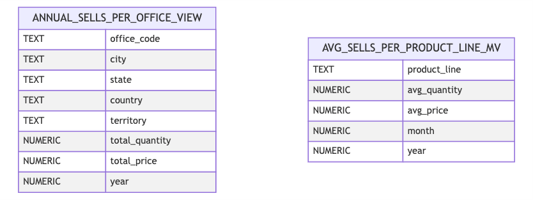
2.1.5. Create a new schema.yml file in the ./classicmodels_modeling/models/analytical_views/folder. To set the schema for the view annual_sells_per_office_view, copy the following into the file and save changes:
version: 2

models:
  - name: annual_sells_per_office_view
    description: "Annual sells per office view"
    columns:
      - name: office_code
      - name: city
      - name: state
      - name: country
      - name: territory
      - name: total_quantity
      - name: total_price
      - name: year
2.1.6. Open the ./classicmodels_modeling/dbt_project.yml file, and at the bottom of the file add the following key:
analytical_views:
  +materialized: view
  +schema: star_schema
This also ensures that no physical tables are created but only materialized views and that they will be created in the schema named star_schema.
2.2 - Average Sales per Product Line
Now you’ve got a business question about the average sales (in terms of units and price) of each product line per month and year.
2.2.1. This is the query which should answer that question. Review the query and run it:
%%sql
SELECT
    dp.product_line
    , AVG(fct.quantity_ordered) AS avg_quantity
    , AVG(fct.quantity_ordered*fct.product_price) AS avg_price
    , EXTRACT(MONTH FROM fct.order_date) AS month
    , EXTRACT(YEAR FROM fct.order_date) AS year
FROM classicmodels_star_schema.fact_orders AS fct
JOIN classicmodels_star_schema.dim_products AS dp ON dp.product_key = fct.product_key
GROUP BY dp.product_line
    , EXTRACT(MONTH FROM fct.order_date)
    , EXTRACT(YEAR FROM fct.order_date)
ORDER BY
    dp.product_line ASC
    , month ASC
    , year ASC
LIMIT 10
 * postgresql+psycopg2://postgresuser:***@de-c4w4lab1-rds.cd044wq8gkrk.us-east-1.rds.amazonaws.com:5432/postgres
10 rows affected.
| product_line | avg_quantity | avg_price | month | year |
|---|---|---|---|---|
| Classic Cars | 33.4000000000000000 | 3655.2330000000000000 | 1 | 2003 |
| Classic Cars | 35.7666666666666667 | 3892.1016666666666667 | 1 | 2004 |
| Classic Cars | 35.0789473684210526 | 3703.4450000000000000 | 1 | 2005 |
| Classic Cars | 40.0000000000000000 | 6313.6800000000000000 | 2 | 2003 |
| Classic Cars | 34.7878787878787879 | 3775.2809090909090909 | 2 | 2004 |
| Classic Cars | 35.5789473684210526 | 3913.0457894736842105 | 2 | 2005 |
| Classic Cars | 35.7307692307692308 | 3734.1607692307692308 | 3 | 2003 |
| Classic Cars | 40.8823529411764706 | 4802.2782352941176471 | 3 | 2004 |
| Classic Cars | 35.4814814814814815 | 3833.0974074074074074 | 3 | 2005 |
| Classic Cars | 38.7500000000000000 | 4795.4350000000000000 | 4 | 2003 |
2.2.2. In the folder ./classicmodels_modeling/models/analytical_views/ create a new file avg_sells_per_product_line_view.sql. Copy the query from the previous step into that file (do not include the lines %%sql and LIMIT 10).
2.2.3. At the beginning of this file right before your query, add the following jinja configuration that creates views instead of physical tables:
2.2.4. Exchange the classicmodels_star_schema with the jinja templating string `` (in two places). Save changes.
2.2.5. In the ./classicmodels_modeling/models/analytical_views/schema.yml file add the schema for the view avg_sells_per_product_line_view:
  - name: avg_sells_per_product_line_view
    description: "Average sells per product lind view"
    columns:
      - name: product_line
      - name: avg_quantity
      - name: avg_price
      - name: month
      - name: year
Save changes.
2.3 - Running Analytical Views
In order to run the analytical views that you just created.
2.3.1. Get back to your dbt project folder classicmodels_modeling run the analytical view:
Note: You may need to reactivate the environment:
source jupyterlab-venv/bin/activate
cd classicmodels_modeling
dbt run -s analytical_views
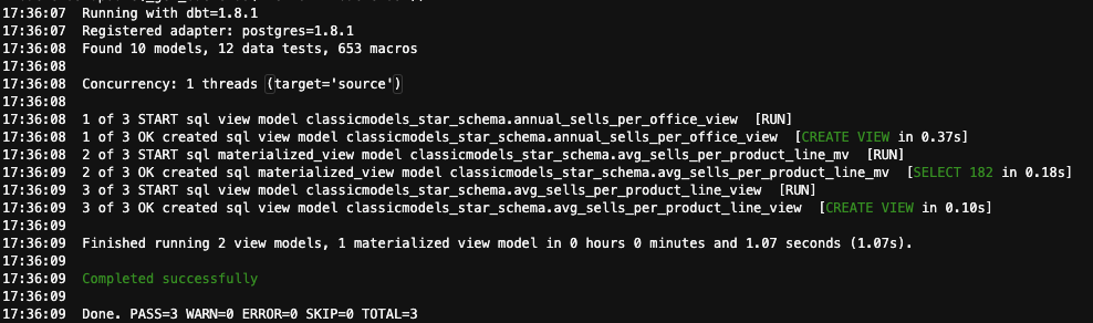
You should see an output similar to this one:
2.3.2. The views will be created at the classicmodels_star_schema database, so you can use the following scripts to check that they were populated:
%%sql
SELECT COUNT(*) FROM classicmodels_star_schema.annual_sells_per_office_view;
 * postgresql+psycopg2://postgresuser:***@de-c4w4lab1-rds.cd044wq8gkrk.us-east-1.rds.amazonaws.com:5432/postgres
1 rows affected.
| count |
|---|
| 21 |
%%sql
SELECT * FROM classicmodels_star_schema.annual_sells_per_office_view order by year desc;
 * postgresql+psycopg2://postgresuser:***@de-c4w4lab1-rds.cd044wq8gkrk.us-east-1.rds.amazonaws.com:5432/postgres
21 rows affected.
| office_key | city | state | country | territory | total_quantity | total_price | year |
|---|---|---|---|---|---|---|---|
| eccbc87e4b5ce2fe28308fd9f2a7baf3 | NYC | NY | USA | NA | 1111 | 101096.20 | 2005 |
| a87ff679a2f3e71d9181a67b7542122c | Paris | None | France | EMEA | 7222 | 648571.84 | 2005 |
| c81e728d9d4c2f636f067f89cc14862c | Boston | MA | USA | NA | 1389 | 123580.17 | 2005 |
| c4ca4238a0b923820dcc509a6f75849b | San Francisco | CA | USA | NA | 4062 | 378973.82 | 2005 |
| 1679091c5a880faf6fb5e6087eb1b2dc | Sydney | NSW | Australia | APAC | 3411 | 299231.22 | 2005 |
| 8f14e45fceea167a5a36dedd4bea2543 | London | None | UK | EMEA | 2015 | 181384.24 | 2005 |
| e4da3b7fbbce2345d7772b0674a318d5 | Tokyo | Chiyoda-Ku | Japan | Japan | 380 | 38099.22 | 2005 |
| c4ca4238a0b923820dcc509a6f75849b | San Francisco | CA | USA | NA | 5697 | 517408.62 | 2004 |
| 1679091c5a880faf6fb5e6087eb1b2dc | Sydney | NSW | Australia | APAC | 5938 | 542996.02 | 2004 |
| 8f14e45fceea167a5a36dedd4bea2543 | London | None | UK | EMEA | 7659 | 706014.52 | 2004 |
| a87ff679a2f3e71d9181a67b7542122c | Paris | None | France | EMEA | 15971 | 1465229.84 | 2004 |
| c81e728d9d4c2f636f067f89cc14862c | Boston | MA | USA | NA | 5101 | 467177.07 | 2004 |
| e4da3b7fbbce2345d7772b0674a318d5 | Tokyo | Chiyoda-Ku | Japan | Japan | 1692 | 151761.45 | 2004 |
| eccbc87e4b5ce2fe28308fd9f2a7baf3 | NYC | NY | USA | NA | 7429 | 665317.99 | 2004 |
| c4ca4238a0b923820dcc509a6f75849b | San Francisco | CA | USA | NA | 6151 | 532681.13 | 2003 |
| e4da3b7fbbce2345d7772b0674a318d5 | Tokyo | Chiyoda-Ku | Japan | Japan | 2851 | 267249.40 | 2003 |
| 8f14e45fceea167a5a36dedd4bea2543 | London | None | UK | EMEA | 6017 | 549551.94 | 2003 |
| a87ff679a2f3e71d9181a67b7542122c | Paris | None | France | EMEA | 10694 | 969959.90 | 2003 |
| 1679091c5a880faf6fb5e6087eb1b2dc | Sydney | NSW | Australia | APAC | 3529 | 304949.11 | 2003 |
| c81e728d9d4c2f636f067f89cc14862c | Boston | MA | USA | NA | 3298 | 301781.38 | 2003 |
| eccbc87e4b5ce2fe28308fd9f2a7baf3 | NYC | NY | USA | NA | 3899 | 391175.53 | 2003 |
%%sql
SELECT COUNT(*) FROM classicmodels_star_schema.avg_sells_per_product_line_view;
 * postgresql+psycopg2://postgresuser:***@de-c4w4lab1-rds.cd044wq8gkrk.us-east-1.rds.amazonaws.com:5432/postgres
1 rows affected.
| count |
|---|
| 182 |
%%sql
SELECT * FROM classicmodels_star_schema.avg_sells_per_product_line_view order by year desc, month asc LIMIT 20;
 * postgresql+psycopg2://postgresuser:***@de-c4w4lab1-rds.cd044wq8gkrk.us-east-1.rds.amazonaws.com:5432/postgres
20 rows affected.
| product_line | avg_quantity | avg_price | month | year |
|---|---|---|---|---|
| Trucks and Buses | 30.6363636363636364 | 2961.0381818181818182 | 1 | 2005 |
| Ships | 35.5555555555555556 | 2695.2244444444444444 | 1 | 2005 |
| Planes | 35.0000000000000000 | 2569.7620000000000000 | 1 | 2005 |
| Classic Cars | 35.0789473684210526 | 3703.4450000000000000 | 1 | 2005 |
| Vintage Cars | 35.1818181818181818 | 2841.6240909090909091 | 1 | 2005 |
| Trains | 26.3333333333333333 | 1753.6266666666666667 | 1 | 2005 |
| Motorcycles | 34.2727272727272727 | 2686.5681818181818182 | 1 | 2005 |
| Motorcycles | 33.0000000000000000 | 2985.6361538461538462 | 2 | 2005 |
| Classic Cars | 35.5789473684210526 | 3913.0457894736842105 | 2 | 2005 |
| Ships | 34.0000000000000000 | 2743.3666666666666667 | 2 | 2005 |
| Planes | 38.5714285714285714 | 3219.5900000000000000 | 2 | 2005 |
| Trains | 36.0000000000000000 | 2161.5600000000000000 | 2 | 2005 |
| Trucks and Buses | 32.3636363636363636 | 3011.4427272727272727 | 2 | 2005 |
| Vintage Cars | 35.2727272727272727 | 2695.6990909090909091 | 2 | 2005 |
| Trucks and Buses | 36.0000000000000000 | 3239.5972727272727273 | 3 | 2005 |
| Trains | 33.0000000000000000 | 2163.2300000000000000 | 3 | 2005 |
| Motorcycles | 39.4615384615384615 | 3386.0776923076923077 | 3 | 2005 |
| Classic Cars | 35.4814814814814815 | 3833.0974074074074074 | 3 | 2005 |
| Planes | 36.7916666666666667 | 2846.5420833333333333 | 3 | 2005 |
| Ships | 36.3333333333333333 | 2702.4400000000000000 | 3 | 2005 |
2.4 - Creating Materialized View
Up to this moment, you have created views. Remember that those views are virtual tables that do not store data physically. Let’s take the last view and create a materialized view so we can compare how these two materialization strategies work in a database.
2.4.1. Take the file ./classicmodels_modeling/models/analytical_views/avg_sells_per_product_line_view.sql, copy it and rename as avg_sells_per_product_line_mv.sql. Open this new file and change the configuration to
Take a look at the value of the materialized key. This value indicates that the materialization strategy will create an actual materialized view, which actually stores data physically.
Save changes.
2.4.2. Open the ./classicmodels_modeling/models/analytical_views/schema.yml file and add a schema named avg_sells_per_product_line_mv for this materialized view:
  - name: avg_sells_per_product_line_mv
    description: "Average sells per product line materialized view"
    columns:
      - name: product_line
      - name: avg_quantity
      - name: avg_price
      - name: month
      - name: year
Save changes.
2.4.3. Finally, run again your dbt process with
dbt run -s analytical_views
Note: Remember that in the dbt_project file, you set this configuration:
analytical_views:
    +materialized: view
    +schema: star_schema
Although this configuration specifies that the materialization strategy is a view, the configuration that you set at the avg_sells_per_product_line_mv.sql file overwrites this configuration to create a materialized view.
2.4.4. Run this command to check that the data has been successfully loaded into the materialized view:
%%sql
SELECT COUNT(*) FROM classicmodels_star_schema.avg_sells_per_product_line_mv;
 * postgresql+psycopg2://postgresuser:***@de-c4w4lab1-rds.cd044wq8gkrk.us-east-1.rds.amazonaws.com:5432/postgres
1 rows affected.
| count |
|---|
| 182 |
%%sql
SELECT * FROM classicmodels_star_schema.avg_sells_per_product_line_mv order by year desc, month asc LIMIT 20;
 * postgresql+psycopg2://postgresuser:***@de-c4w4lab1-rds.cd044wq8gkrk.us-east-1.rds.amazonaws.com:5432/postgres
20 rows affected.
| product_line | avg_quantity | avg_price | month | year |
|---|---|---|---|---|
| Trucks and Buses | 30.6363636363636364 | 2961.0381818181818182 | 1 | 2005 |
| Ships | 35.5555555555555556 | 2695.2244444444444444 | 1 | 2005 |
| Planes | 35.0000000000000000 | 2569.7620000000000000 | 1 | 2005 |
| Classic Cars | 35.0789473684210526 | 3703.4450000000000000 | 1 | 2005 |
| Vintage Cars | 35.1818181818181818 | 2841.6240909090909091 | 1 | 2005 |
| Trains | 26.3333333333333333 | 1753.6266666666666667 | 1 | 2005 |
| Motorcycles | 34.2727272727272727 | 2686.5681818181818182 | 1 | 2005 |
| Motorcycles | 33.0000000000000000 | 2985.6361538461538462 | 2 | 2005 |
| Classic Cars | 35.5789473684210526 | 3913.0457894736842105 | 2 | 2005 |
| Ships | 34.0000000000000000 | 2743.3666666666666667 | 2 | 2005 |
| Planes | 38.5714285714285714 | 3219.5900000000000000 | 2 | 2005 |
| Trains | 36.0000000000000000 | 2161.5600000000000000 | 2 | 2005 |
| Trucks and Buses | 32.3636363636363636 | 3011.4427272727272727 | 2 | 2005 |
| Vintage Cars | 35.2727272727272727 | 2695.6990909090909091 | 2 | 2005 |
| Trucks and Buses | 36.0000000000000000 | 3239.5972727272727273 | 3 | 2005 |
| Trains | 33.0000000000000000 | 2163.2300000000000000 | 3 | 2005 |
| Motorcycles | 39.4615384615384615 | 3386.0776923076923077 | 3 | 2005 |
| Classic Cars | 35.4814814814814815 | 3833.0974074074074074 | 3 | 2005 |
| Planes | 36.7916666666666667 | 2846.5420833333333333 | 3 | 2005 |
| Ships | 36.3333333333333333 | 2702.4400000000000000 | 3 | 2005 |
Now, it is the time to actually understand the difference between views and materialized views. Given that materialized views store data physically, they need to be refreshed when the underlying tables are updated. On the other hand, as views require the execution of the underlying query, they will always present up-to-date data.
2.4.5. Let’s insert some mock data into the fact_orders table and see how it affects the views and materialized views. Execute the following cell to insert the data. Take a look at the dates, as all of them are in the year 2006 while the maximum year we have in our database currently is 2005.
%%sql
SELECT MAX(EXTRACT(YEAR FROM fct.order_date))
FROM classicmodels_star_schema.fact_orders fct;
 * postgresql+psycopg2://postgresuser:***@de-c4w4lab1-rds.cd044wq8gkrk.us-east-1.rds.amazonaws.com:5432/postgres
1 rows affected.
| max |
|---|
| 2005 |
%%sql
INSERT INTO classicmodels_star_schema.fact_orders (fact_order_key, customer_key, employee_key, office_key, product_key, order_date, order_required_date, order_shipped_date, quantity_ordered, product_price) VALUES ('9eec411e690b55dafeb3ec3393aa6d57', '7d04bbbe5494ae9d2f5a76aa1c00fa2f', '4671aeaf49c792689533b00664a5c3ef', 'eccbc87e4b5ce2fe28308fd9f2a7baf3', '296efc252c7855537b5d9e6015bf42b8', '2006-06-01 00:00:00', '2006-07-01 00:00:00', '2006-06-15 00:00:00', 41, 83.79);
INSERT INTO classicmodels_star_schema.fact_orders (fact_order_key, customer_key, employee_key, office_key, product_key, order_date, order_required_date, order_shipped_date, quantity_ordered, product_price) VALUES ('f485cfdd94901e9e237dcc3f644f7edc', '7d04bbbe5494ae9d2f5a76aa1c00fa2f', '4671aeaf49c792689533b00664a5c3ef', 'eccbc87e4b5ce2fe28308fd9f2a7baf3', '8bff119b349bf271ef0684a15808ea18', '2006-06-01 00:00:00', '2006-07-01 00:00:00', '2006-06-15 00:00:00', 11, 50.32);
INSERT INTO classicmodels_star_schema.fact_orders (fact_order_key, customer_key, employee_key, office_key, product_key, order_date, order_required_date, order_shipped_date, quantity_ordered, product_price) VALUES ('7eecd924b84c4a03fcb69d5ec6df4670', '0f28b5d49b3020afeecd95b4009adf4c', 'd1ee59e20ad01cedc15f5118a7626099', 'a87ff679a2f3e71d9181a67b7542122c', '99733605e1ea651ec564248e05f77741', '2006-06-02 00:00:00', '2006-06-21 00:00:00', '2006-06-07 00:00:00', 18, 94.92 );
 * postgresql+psycopg2://postgresuser:***@de-c4w4lab1-rds.cd044wq8gkrk.us-east-1.rds.amazonaws.com:5432/postgres
1 rows affected.
1 rows affected.
1 rows affected.


[]
2.4.6. Now that you have inserted the data, query again the views. Remember that annual_sells_per_office_view had 21 rows while avg_sells_per_product_line_view had 182 rows before the update.
%%sql
SELECT COUNT(*) FROM classicmodels_star_schema.annual_sells_per_office_view;
 * postgresql+psycopg2://postgresuser:***@de-c4w4lab1-rds.cd044wq8gkrk.us-east-1.rds.amazonaws.com:5432/postgres
1 rows affected.
| count |
|---|
| 23 |
%%sql
SELECT * FROM classicmodels_star_schema.annual_sells_per_office_view order by year desc;
 * postgresql+psycopg2://postgresuser:***@de-c4w4lab1-rds.cd044wq8gkrk.us-east-1.rds.amazonaws.com:5432/postgres
23 rows affected.
| office_key | city | state | country | territory | total_quantity | total_price | year |
|---|---|---|---|---|---|---|---|
| eccbc87e4b5ce2fe28308fd9f2a7baf3 | NYC | NY | USA | NA | 52 | 3988.91 | 2006 |
| a87ff679a2f3e71d9181a67b7542122c | Paris | None | France | EMEA | 18 | 1708.56 | 2006 |
| c81e728d9d4c2f636f067f89cc14862c | Boston | MA | USA | NA | 1389 | 123580.17 | 2005 |
| c4ca4238a0b923820dcc509a6f75849b | San Francisco | CA | USA | NA | 4062 | 378973.82 | 2005 |
| 1679091c5a880faf6fb5e6087eb1b2dc | Sydney | NSW | Australia | APAC | 3411 | 299231.22 | 2005 |
| 8f14e45fceea167a5a36dedd4bea2543 | London | None | UK | EMEA | 2015 | 181384.24 | 2005 |
| eccbc87e4b5ce2fe28308fd9f2a7baf3 | NYC | NY | USA | NA | 1111 | 101096.20 | 2005 |
| a87ff679a2f3e71d9181a67b7542122c | Paris | None | France | EMEA | 7222 | 648571.84 | 2005 |
| e4da3b7fbbce2345d7772b0674a318d5 | Tokyo | Chiyoda-Ku | Japan | Japan | 380 | 38099.22 | 2005 |
| c4ca4238a0b923820dcc509a6f75849b | San Francisco | CA | USA | NA | 5697 | 517408.62 | 2004 |
| 1679091c5a880faf6fb5e6087eb1b2dc | Sydney | NSW | Australia | APAC | 5938 | 542996.02 | 2004 |
| 8f14e45fceea167a5a36dedd4bea2543 | London | None | UK | EMEA | 7659 | 706014.52 | 2004 |
| a87ff679a2f3e71d9181a67b7542122c | Paris | None | France | EMEA | 15971 | 1465229.84 | 2004 |
| c81e728d9d4c2f636f067f89cc14862c | Boston | MA | USA | NA | 5101 | 467177.07 | 2004 |
| e4da3b7fbbce2345d7772b0674a318d5 | Tokyo | Chiyoda-Ku | Japan | Japan | 1692 | 151761.45 | 2004 |
| eccbc87e4b5ce2fe28308fd9f2a7baf3 | NYC | NY | USA | NA | 7429 | 665317.99 | 2004 |
| e4da3b7fbbce2345d7772b0674a318d5 | Tokyo | Chiyoda-Ku | Japan | Japan | 2851 | 267249.40 | 2003 |
| a87ff679a2f3e71d9181a67b7542122c | Paris | None | France | EMEA | 10694 | 969959.90 | 2003 |
| c4ca4238a0b923820dcc509a6f75849b | San Francisco | CA | USA | NA | 6151 | 532681.13 | 2003 |
| eccbc87e4b5ce2fe28308fd9f2a7baf3 | NYC | NY | USA | NA | 3899 | 391175.53 | 2003 |
| c81e728d9d4c2f636f067f89cc14862c | Boston | MA | USA | NA | 3298 | 301781.38 | 2003 |
| 8f14e45fceea167a5a36dedd4bea2543 | London | None | UK | EMEA | 6017 | 549551.94 | 2003 |
| 1679091c5a880faf6fb5e6087eb1b2dc | Sydney | NSW | Australia | APAC | 3529 | 304949.11 | 2003 |
%%sql
SELECT COUNT(*) FROM classicmodels_star_schema.avg_sells_per_product_line_view;
 * postgresql+psycopg2://postgresuser:***@de-c4w4lab1-rds.cd044wq8gkrk.us-east-1.rds.amazonaws.com:5432/postgres
1 rows affected.
| count |
|---|
| 183 |
%%sql
SELECT * FROM classicmodels_star_schema.avg_sells_per_product_line_view order by year desc, month asc LIMIT 20;
 * postgresql+psycopg2://postgresuser:***@de-c4w4lab1-rds.cd044wq8gkrk.us-east-1.rds.amazonaws.com:5432/postgres
20 rows affected.
| product_line | avg_quantity | avg_price | month | year |
|---|---|---|---|---|
| Trucks and Buses | 23.3333333333333333 | 1899.1566666666666667 | 6 | 2006 |
| Trains | 26.3333333333333333 | 1753.6266666666666667 | 1 | 2005 |
| Vintage Cars | 35.1818181818181818 | 2841.6240909090909091 | 1 | 2005 |
| Planes | 35.0000000000000000 | 2569.7620000000000000 | 1 | 2005 |
| Classic Cars | 35.0789473684210526 | 3703.4450000000000000 | 1 | 2005 |
| Trucks and Buses | 30.6363636363636364 | 2961.0381818181818182 | 1 | 2005 |
| Ships | 35.5555555555555556 | 2695.2244444444444444 | 1 | 2005 |
| Motorcycles | 34.2727272727272727 | 2686.5681818181818182 | 1 | 2005 |
| Classic Cars | 35.5789473684210526 | 3913.0457894736842105 | 2 | 2005 |
| Planes | 38.5714285714285714 | 3219.5900000000000000 | 2 | 2005 |
| Ships | 34.0000000000000000 | 2743.3666666666666667 | 2 | 2005 |
| Vintage Cars | 35.2727272727272727 | 2695.6990909090909091 | 2 | 2005 |
| Trains | 36.0000000000000000 | 2161.5600000000000000 | 2 | 2005 |
| Motorcycles | 33.0000000000000000 | 2985.6361538461538462 | 2 | 2005 |
| Trucks and Buses | 32.3636363636363636 | 3011.4427272727272727 | 2 | 2005 |
| Trucks and Buses | 36.0000000000000000 | 3239.5972727272727273 | 3 | 2005 |
| Trains | 33.0000000000000000 | 2163.2300000000000000 | 3 | 2005 |
| Motorcycles | 39.4615384615384615 | 3386.0776923076923077 | 3 | 2005 |
| Classic Cars | 35.4814814814814815 | 3833.0974074074074074 | 3 | 2005 |
| Planes | 36.7916666666666667 | 2846.5420833333333333 | 3 | 2005 |
2.4.7. Finally, let’s query the materialized view. What can you see?
%%sql
SELECT COUNT(*) FROM classicmodels_star_schema.avg_sells_per_product_line_mv;
 * postgresql+psycopg2://postgresuser:***@de-c4w4lab1-rds.cd044wq8gkrk.us-east-1.rds.amazonaws.com:5432/postgres
1 rows affected.
| count |
|---|
| 182 |
%%sql
SELECT * FROM classicmodels_star_schema.avg_sells_per_product_line_mv order by year desc, month asc LIMIT 20;
 * postgresql+psycopg2://postgresuser:***@de-c4w4lab1-rds.cd044wq8gkrk.us-east-1.rds.amazonaws.com:5432/postgres
20 rows affected.
| product_line | avg_quantity | avg_price | month | year |
|---|---|---|---|---|
| Trucks and Buses | 30.6363636363636364 | 2961.0381818181818182 | 1 | 2005 |
| Ships | 35.5555555555555556 | 2695.2244444444444444 | 1 | 2005 |
| Planes | 35.0000000000000000 | 2569.7620000000000000 | 1 | 2005 |
| Classic Cars | 35.0789473684210526 | 3703.4450000000000000 | 1 | 2005 |
| Vintage Cars | 35.1818181818181818 | 2841.6240909090909091 | 1 | 2005 |
| Trains | 26.3333333333333333 | 1753.6266666666666667 | 1 | 2005 |
| Motorcycles | 34.2727272727272727 | 2686.5681818181818182 | 1 | 2005 |
| Motorcycles | 33.0000000000000000 | 2985.6361538461538462 | 2 | 2005 |
| Classic Cars | 35.5789473684210526 | 3913.0457894736842105 | 2 | 2005 |
| Ships | 34.0000000000000000 | 2743.3666666666666667 | 2 | 2005 |
| Planes | 38.5714285714285714 | 3219.5900000000000000 | 2 | 2005 |
| Trains | 36.0000000000000000 | 2161.5600000000000000 | 2 | 2005 |
| Trucks and Buses | 32.3636363636363636 | 3011.4427272727272727 | 2 | 2005 |
| Vintage Cars | 35.2727272727272727 | 2695.6990909090909091 | 2 | 2005 |
| Trucks and Buses | 36.0000000000000000 | 3239.5972727272727273 | 3 | 2005 |
| Trains | 33.0000000000000000 | 2163.2300000000000000 | 3 | 2005 |
| Motorcycles | 39.4615384615384615 | 3386.0776923076923077 | 3 | 2005 |
| Classic Cars | 35.4814814814814815 | 3833.0974074074074074 | 3 | 2005 |
| Planes | 36.7916666666666667 | 2846.5420833333333333 | 3 | 2005 |
| Ships | 36.3333333333333333 | 2702.4400000000000000 | 3 | 2005 |
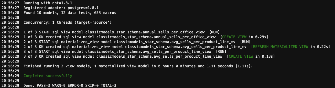
When querying the materialized view, you can see that you get the same number of rows as before the update to the fact_orders table. In order to refresh this materialized view, you should run again the dbt model. Do it with the command
dbt run -s analytical_views
You will see that the materialized view has been refreshed:
Finally, query again your materialized view to see the difference.
%%sql
SELECT COUNT(*) FROM classicmodels_star_schema.avg_sells_per_product_line_mv;
 * postgresql+psycopg2://postgresuser:***@de-c4w4lab1-rds.cd044wq8gkrk.us-east-1.rds.amazonaws.com:5432/postgres
1 rows affected.
| count |
|---|
| 183 |
%%sql
SELECT * FROM classicmodels_star_schema.avg_sells_per_product_line_mv order by year desc, month asc LIMIT 20;
 * postgresql+psycopg2://postgresuser:***@de-c4w4lab1-rds.cd044wq8gkrk.us-east-1.rds.amazonaws.com:5432/postgres
20 rows affected.
| product_line | avg_quantity | avg_price | month | year |
|---|---|---|---|---|
| Trucks and Buses | 23.3333333333333333 | 1899.1566666666666667 | 6 | 2006 |
| Trains | 26.3333333333333333 | 1753.6266666666666667 | 1 | 2005 |
| Vintage Cars | 35.1818181818181818 | 2841.6240909090909091 | 1 | 2005 |
| Planes | 35.0000000000000000 | 2569.7620000000000000 | 1 | 2005 |
| Classic Cars | 35.0789473684210526 | 3703.4450000000000000 | 1 | 2005 |
| Trucks and Buses | 30.6363636363636364 | 2961.0381818181818182 | 1 | 2005 |
| Ships | 35.5555555555555556 | 2695.2244444444444444 | 1 | 2005 |
| Motorcycles | 34.2727272727272727 | 2686.5681818181818182 | 1 | 2005 |
| Classic Cars | 35.5789473684210526 | 3913.0457894736842105 | 2 | 2005 |
| Planes | 38.5714285714285714 | 3219.5900000000000000 | 2 | 2005 |
| Ships | 34.0000000000000000 | 2743.3666666666666667 | 2 | 2005 |
| Vintage Cars | 35.2727272727272727 | 2695.6990909090909091 | 2 | 2005 |
| Trains | 36.0000000000000000 | 2161.5600000000000000 | 2 | 2005 |
| Motorcycles | 33.0000000000000000 | 2985.6361538461538462 | 2 | 2005 |
| Trucks and Buses | 32.3636363636363636 | 3011.4427272727272727 | 2 | 2005 |
| Trucks and Buses | 36.0000000000000000 | 3239.5972727272727273 | 3 | 2005 |
| Trains | 33.0000000000000000 | 2163.2300000000000000 | 3 | 2005 |
| Motorcycles | 39.4615384615384615 | 3386.0776923076923077 | 3 | 2005 |
| Classic Cars | 35.4814814814814815 | 3833.0974074074074074 | 3 | 2005 |
| Planes | 36.7916666666666667 | 2846.5420833333333333 | 3 | 2005 |
With that exercise, you can notice the difference between a view and a materialized view. You may be wondering when you should use one or the other and you can use these paragraphs as a hint:
-
Views: Use when you need a simple way to encapsulate complex queries, enhance security by exposing only certain data, or provide a simplified interface to the underlying tables. Ideal for frequently changing data where up-to-the-moment accuracy is essential.
-
Materialized Views: Use when you need to improve performance for complex, resource-intensive queries. Ideal for reporting and data warehousing scenarios where data does not need to be up-to-the-second accurate, and where the performance gain from precomputed results outweighs the need for real-time data.
3 - Dashboard with Apache Superset
Note:Apache Superset takes around 15 to 20 minutes to load from the start of the lab, if you don’t see the interface when entering the URL in a new tab, wait a while and refresh the page.
3.1. The EC2 instance has been set up for you to work with Apache Superset, the URL is among the CloudFormation Outputs. Access the Superset UI using the URL provided in the CloudFormation Outputs (take the value for the key SupersetEndpoint), you should see a login screen like this:
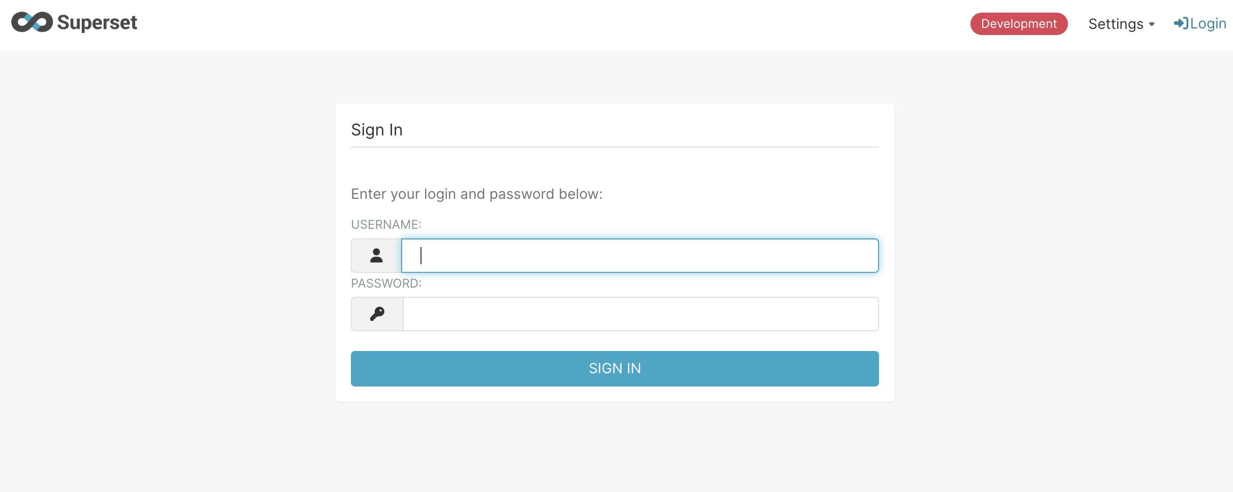
3.2. Login using the following credentials:
- user:
admin - password:
admin
3.3. Configure the Postgres connection. Click on the dropdown Settings menu in the top right, and under the Data section select Database Connections. Click on the top right + Database button, a new menu should appear to configure the new connection:
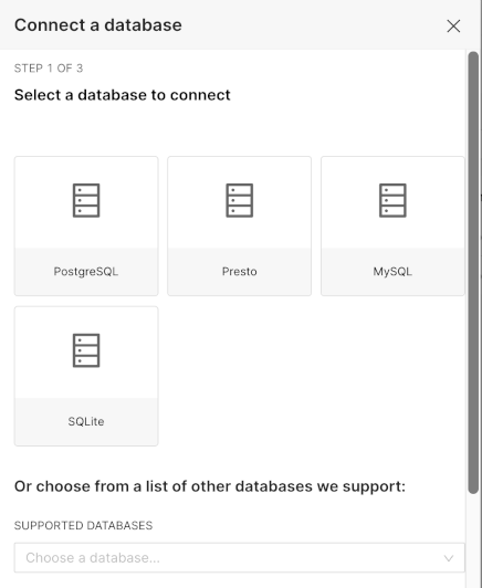
Select PostgreSQL and click Next. Fill out the details using the same connection parameters as the ones found in the ./scripts/profiles.yml. The details for the connection are also can be printed out:
print(DBCONFIG)
After filling out the details, click on Connect button, this should have created a new connection in the Data Connections section. Click on Finish button.
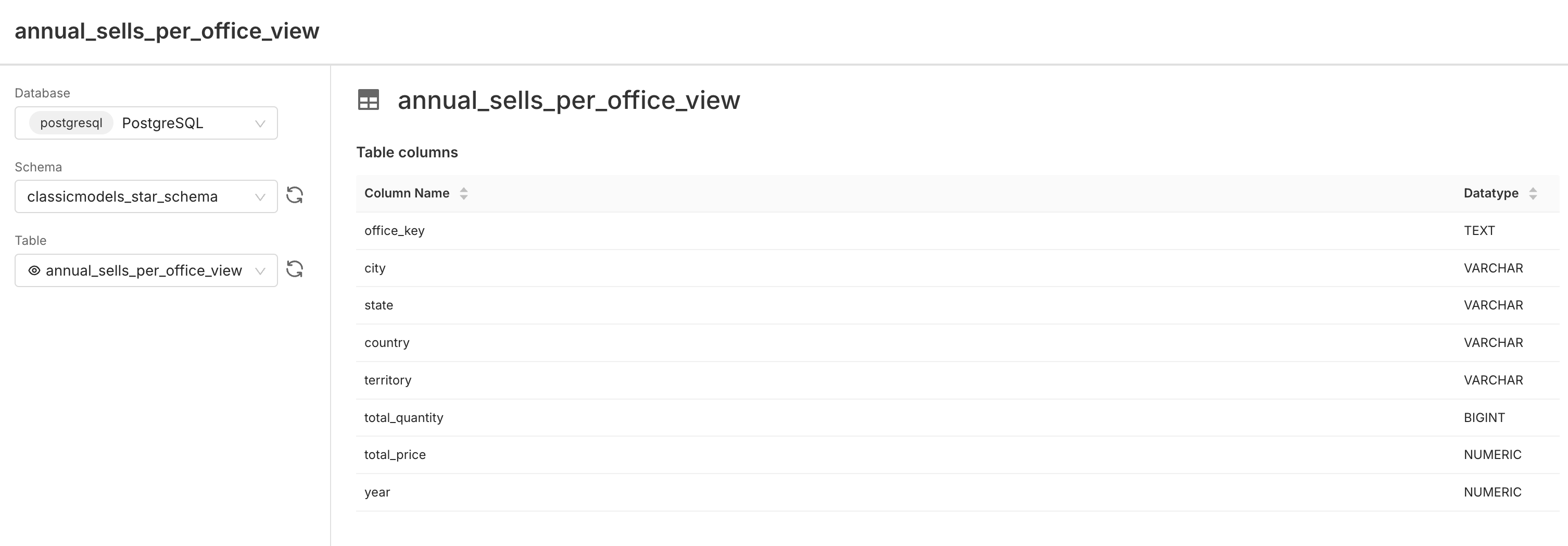
3.4. Now, select the Datasets tab in the top header menu. You will be directed to a page with various example datasets. Click on + DATASET button on the top right, a new screen will appear, you can use the connection that you just configured for Postgres, then select the classicmodels_star_schema and finally one of the views:
3.5. Click on the CREATE DATASET AND CREATE CHART button (in the bottom right), you will be directed to a new page to create a chart based on the dataset. You can select the type of chart and what variable is used for each dimension.
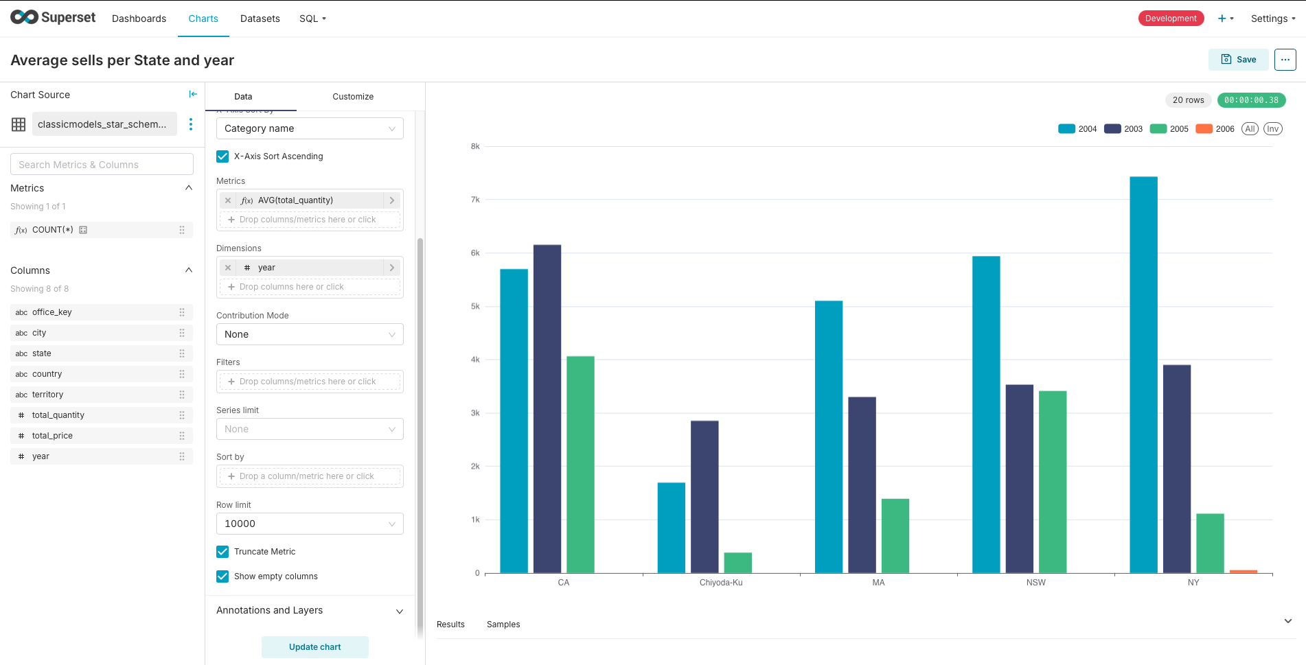
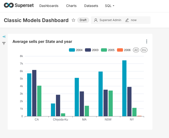
Once you are done with the chart, hit the Save button on the top right, it will ask you to give the chart a name and then save it. Create a chart for each view then create a new dashboard in the Dashboards section of the top navigational header, using the + Dashboard button. Enter a name (in the top left part) for your dashboard and then drag and drop the charts you created earlier onto the dashboard canvas, Resize and arrange the charts as desired to create your dashboard layout and finally click Save to save your dashboard layout.
In this lab, you focused on data visualization using various types of views and a dashboard tool. Effective visual communication is crucial for presenting your findings and the results of your data pipelines to potential stakeholders. Although this task aligns more with the role of a data analyst, it is essential to understand their responsibilities and how we can supply them with the necessary data for their work.