coursera-data-engineering
Capstone Project Part 1 - ETL and Data Modeling
During this capstone project, you will develop a data pipeline as part of a new project in the company DeFtunes. You will showcase the abilities and tools you have been using during the whole specialization.
Table of Contents
- 1 - Introduction
- 2 - Data Sources
- 3 - Exploratory Data Analysis
- 4 - ETL Pipeline with AWS Glue and Terraform
- 5 - Data Modeling with dbt and Redshift Spectrum
- 6 - Upload Files for Grading
1 - Introduction
DeFtunes is a new company in the music industry, offering a subscription-based app for streaming songs. Recently, they have expanded their services to include digital song purchases. With this new retail feature, DeFtunes requires a data pipeline to extract purchase data from their new API and operational database, enrich and model this data, and ultimately deliver the comprehensive data model for the Data Analysis team to review and gain insights. Your task is to develop this pipeline, ensuring the data is accurately processed and ready for in-depth analysis.
Here is the diagram with the main requirements for this project:
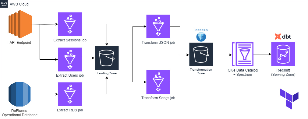
- The pipeline has to follow a medallion architecture with a landing, transform and serving zone.
- The data generated in the pipeline will be stored in the company’s data lake, in this case, an S3 bucket.
- The silver layer should use Iceberg tables, and the gold layer should be inside Redshift.
- The pipeline should be reproducible, you will have to implement it using Terraform.
- The data should be modelled into a star schema in the serving layer, you should use dbt for the modelling part.
Before starting, you will need to import some required libraries and modules for the capstone development.
import json
import requests
import pandas as pd
import subprocess

%load_ext sql

LAB_PREFIX='de-c4w4a1'
2 - Data Sources
The first data source you will be using is the DeFtunes operational database, which is running in RDS with a Postgres engine. This database contains a table with all the relevant information for the available songs that you can purchase. Let’s connect to the table using the %sql magic.
2.1. To define the connection string, go to CloudFormation Outputs in the AWS console. You will see the key PostgresEndpoint, copy the corresponding Value and replace with it the placeholder <POSTGRES_ENDPOINT> in the cell below (please, replace the whole placeholder including the brackets <>). Then run the cell code.
RDSDBHOST = 'de-c4w4a1-rds.clgg68y6ow15.us-east-1.rds.amazonaws.com'
RDSDBPORT = '5432'
RDSDBNAME = 'postgres'
RDSDBUSER = 'postgresuser'
RDSDBPASSWORD = 'adminpwrd'

postgres_connection_url = f'postgresql+psycopg2://{RDSDBUSER}:{RDSDBPASSWORD}@{RDSDBHOST}:{RDSDBPORT}/{RDSDBNAME}'
%sql {postgres_connection_url}
2.2. Test that the connection works by running the following query.
%%sql
SELECT schema_name
FROM information_schema.schemata;
 * postgresql+psycopg2://postgresuser:***@de-c4w4a1-rds.clgg68y6ow15.us-east-1.rds.amazonaws.com:5432/postgres
6 rows affected.
| schema_name |
|---|
| public |
| aws_s3 |
| aws_commons |
| deftunes |
| information_schema |
| pg_catalog |
2.3. Inside the deftunes schema there is a table songs which was mentioned before. Let’s query a sample from it:
Note: The songs table is based on the Million Song Dataset, more information can be found here.
%%sql
SELECT *
FROM deftunes.songs
LIMIT 5;
 * postgresql+psycopg2://postgresuser:***@de-c4w4a1-rds.clgg68y6ow15.us-east-1.rds.amazonaws.com:5432/postgres
5 rows affected.
| track_id | title | song_id | release | artist_id | artist_mbid | artist_name | duration | artist_familiarity | artist_hotttnesss | year | track_7digitalid | shs_perf | shs_work |
|---|---|---|---|---|---|---|---|---|---|---|---|---|---|
| TRMBFJC12903CE2A89 | Mystery Babylon | SOGOPFY12AB018E5B1 | Healing of All Nations | ARP06GY1187B98B0F0 | 106e0414-95a7-45e9-8176-bbc938deed68 | Yami Bolo | 146.49425 | 0.4955022 | 0.3224826 | 2001 | 8562838 | -1 | 0 |
| TRMBFTN128F42665EA | Världen É Din | SOKFZOR12A8C1306B0 | Omérta | ARZ6UKQ1187B9B0E35 | a432b2e7-7598-419b-8760-e8accff3c725 | The Latin Kings | 268.22485 | 0.54002666 | 0.42142987 | 0 | 3164205 | -1 | 0 |
| TRMBFUD128F9318502 | Working Underground | SOAVROI12AB0183312 | My Land is Your Land | ARTOD2W1187B99FC16 | 41b79e6f-9621-45c9-836c-9f08bedba4eb | Ashley Hutchings_ Ernesto De Pascale | 226.42892 | 0.4131989 | 0.33407375 | 0 | 3957236 | -1 | 0 |
| TRMBFNG12903CEA2A8 | Alien Bzzing | SOCWCQV12AC3DF9B21 | Uomini D'onore | ARUE65J1187B9AB4D9 | 644feeb5-0ad9-457f-9d29-98474d42d9d3 | Fireside | 345.96527 | 0.48547184 | 0.3672936 | 1997 | 8593681 | -1 | 0 |
| TRMBFSN128F4259499 | Repente | SOGWDNA12A8C139BFC | Limite das Aguas | ARS8WH31187B9B8B04 | e02d67b8-b581-478e-be33-c988627e4050 | Edu Lobo | 269.47873 | 0.34406215 | 0.0 | 0 | 2775420 | -1 | 0 |
2.4. The second data source is a new API designed for the song purchase process. This API contains information on the purchases done by the users of the App and also contains relevant information about each user. Copy the endpoint value from the CloudFormation outputs tab and replace the placeholder <API_ENDPOINT> with it.
API_ENDPOINT = "3.231.170.39:8080"
You can also access the documentation to the API by opening the new browser tab, pasting the API endpoint value and adding /docs to it. You will see an interactive interface to test the API.
2.5. The first endpoint is to the sessions path in the API, which retrieves the transactional sessions. Let’s test the API by performing a GET request to the endpoint with the next cell. If everything works you should get a 200 status code from the sessions_response object.
request_start_date = "2020-01-01"
request_end_date = "2020-03-01"
sessions_response = requests.get(f'http://{API_ENDPOINT}/sessions?start_date={request_start_date}&end_date={request_end_date}')
print(sessions_response.status_code)
200
2.6. You can get the content of the response in JSON format using the .json() method, let’s print the first record with the following cell.
sessions_json = sessions_response.json()
print(json.dumps(sessions_json[0], indent=4))
{
    "user_id": "6b287203-7cab-4f1a-b1a4-2b5076294682",
    "session_id": "04a5e8ac-1acd-48dc-88b9-651c4ddf489c",
    "session_items": [
        {
            "song_id": "TRXKAGX128F9342DD7",
            "song_name": "3 Cards",
            "artist_id": "AR475MP1187B9A5449",
            "artist_name": "The Balancing Act",
            "price": 1.03,
            "currency": "USD",
            "liked": true,
            "liked_since": "2023-01-27T08:29:54.970697"
        },
        {
            "song_id": "TRUKGBT128F4292C9B",
            "song_name": "Parisian Walls (gband Version_ Barcelona)",
            "artist_id": "ARP9HJX1187FB4E5DA",
            "artist_name": "Apostle Of Hustle",
            "price": 1.31,
            "currency": "USD",
            "liked": true,
            "liked_since": "2023-06-14T00:27:55.876873"
        },
        {
            "song_id": "TRCPHWV128F4228647",
            "song_name": "Los Sabanales",
            "artist_id": "ARRLMTZ1187B9AB6DD",
            "artist_name": "Los Corraleros De Majagual",
            "price": 0.69,
            "currency": "USD",
            "liked": false,
            "liked_since": null
        },
        {
            "song_id": "TRMHNOY12903CDD075",
            "song_name": "Earth Messiah",
            "artist_id": "ARHS5PJ1187FB3C50D",
            "artist_name": "Cathedral",
            "price": 0.52,
            "currency": "USD",
            "liked": false,
            "liked_since": null
        },
        {
            "song_id": "TRIBGDZ128F425A019",
            "song_name": "Eu sei que vou te amar",
            "artist_id": "ARJK24L1187B9AFF5E",
            "artist_name": "Quarteto Em Cy",
            "price": 1.74,
            "currency": "USD",
            "liked": false,
            "liked_since": null
        },
        {
            "song_id": "TROJSDS128F146E6E2",
            "song_name": "Write My Ticket",
            "artist_id": "AR227JP1187FB375BC",
            "artist_name": "Tift Merritt",
            "price": 0.76,
            "currency": "USD",
            "liked": true,
            "liked_since": "2023-10-18T21:54:16.351564"
        }
    ],
    "user_agent": "Mozilla/5.0 (Windows NT 11.0) AppleWebKit/531.2 (KHTML, like Gecko) Chrome/19.0.859.0 Safari/531.2",
    "session_start_time": "2020-02-07T18:05:25.824461"
}
2.7. The second endpoint is to the users path in the API, it retrieves the transactional sessions. Perform a GET request to the endpoint with the next cell, then print a sample with the cell after that one.
users_request = requests.get(f'http://{API_ENDPOINT}/users')
print(users_request.status_code)
200
users_json = users_request.json()
print(json.dumps(users_json[0], indent=4))
{
    "user_id": "a3141825-3a8c-4968-a3af-5362011ef7d5",
    "user_name": "Elizabeth",
    "user_lastname": "Carey",
    "user_location": [
        "46.32313",
        "-0.45877",
        "Niort",
        "FR",
        "Europe/Paris"
    ],
    "user_since": "2020-12-22T14:15:35.936090"
}
3 - Exploratory Data Analysis
To better understand the data sources, start analyzing the data types and values that come from each source. You can use the pandas library to perform Exploratory Data Analysis (EDA) on samples of data.
3.1. Let’s begin with the songs table in the source RDS database, we will take advantage of the %sql magic to bring a sample with SQL and convert it into a pandas dataframe.
songs_result = %sql SELECT *FROM deftunes.songs LIMIT 5
songs_df = songs_result.DataFrame()
songs_df.head()
 * postgresql+psycopg2://postgresuser:***@de-c4w4a1-rds.clgg68y6ow15.us-east-1.rds.amazonaws.com:5432/postgres
5 rows affected.
| track_id | title | song_id | release | artist_id | artist_mbid | artist_name | duration | artist_familiarity | artist_hotttnesss | year | track_7digitalid | shs_perf | shs_work | |
|---|---|---|---|---|---|---|---|---|---|---|---|---|---|---|
| 0 | TRMBFJC12903CE2A89 | Mystery Babylon | SOGOPFY12AB018E5B1 | Healing of All Nations | ARP06GY1187B98B0F0 | 106e0414-95a7-45e9-8176-bbc938deed68 | Yami Bolo | 146.49425 | 0.495502 | 0.322483 | 2001 | 8562838 | -1 | 0 |
| 1 | TRMBFTN128F42665EA | Världen É Din | SOKFZOR12A8C1306B0 | Omérta | ARZ6UKQ1187B9B0E35 | a432b2e7-7598-419b-8760-e8accff3c725 | The Latin Kings | 268.22485 | 0.540027 | 0.421430 | 0 | 3164205 | -1 | 0 |
| 2 | TRMBFUD128F9318502 | Working Underground | SOAVROI12AB0183312 | My Land is Your Land | ARTOD2W1187B99FC16 | 41b79e6f-9621-45c9-836c-9f08bedba4eb | Ashley Hutchings_ Ernesto De Pascale | 226.42892 | 0.413199 | 0.334074 | 0 | 3957236 | -1 | 0 |
| 3 | TRMBFNG12903CEA2A8 | Alien Bzzing | SOCWCQV12AC3DF9B21 | Uomini D'onore | ARUE65J1187B9AB4D9 | 644feeb5-0ad9-457f-9d29-98474d42d9d3 | Fireside | 345.96527 | 0.485472 | 0.367294 | 1997 | 8593681 | -1 | 0 |
| 4 | TRMBFSN128F4259499 | Repente | SOGWDNA12A8C139BFC | Limite das Aguas | ARS8WH31187B9B8B04 | e02d67b8-b581-478e-be33-c988627e4050 | Edu Lobo | 269.47873 | 0.344062 | 0.000000 | 0 | 2775420 | -1 | 0 |
3.1. Use Pandas info() method to print out a summary of information about the dataframe, including information about the columns such as their data types.
print(songs_df.info())
<class 'pandas.core.frame.DataFrame'>
RangeIndex: 5 entries, 0 to 4
Data columns (total 14 columns):
 #   Column              Non-Null Count  Dtype
---  ------              --------------  -----
 0   track_id            5 non-null      object
 1   title               5 non-null      object
 2   song_id             5 non-null      object
 3   release             5 non-null      object
 4   artist_id           5 non-null      object
 5   artist_mbid         5 non-null      object
 6   artist_name         5 non-null      object
 7   duration            5 non-null      float64
 8   artist_familiarity  5 non-null      float64
 9   artist_hotttnesss   5 non-null      float64
 10  year                5 non-null      int64
 11  track_7digitalid    5 non-null      int64
 12  shs_perf            5 non-null      int64
 13  shs_work            5 non-null      int64
dtypes: float64(3), int64(4), object(7)
memory usage: 688.0+ bytes
None
3.2. Use the describe() method to generate a summary of statistics about the numerical and object columns in the dataframe.
songs_df.describe()
| duration | artist_familiarity | artist_hotttnesss | year | track_7digitalid | shs_perf | shs_work | |
|---|---|---|---|---|---|---|---|
| count | 5.000000 | 5.000000 | 5.000000 | 5.000000 | 5.000000e+00 | 5.0 | 5.0 |
| mean | 251.318404 | 0.455652 | 0.289056 | 799.600000 | 5.410676e+06 | -1.0 | 0.0 |
| std | 72.768888 | 0.077219 | 0.166088 | 1094.898306 | 2.922813e+06 | 0.0 | 0.0 |
| min | 146.494250 | 0.344062 | 0.000000 | 0.000000 | 2.775420e+06 | -1.0 | 0.0 |
| 25% | 226.428920 | 0.413199 | 0.322483 | 0.000000 | 3.164205e+06 | -1.0 | 0.0 |
| 50% | 268.224850 | 0.485472 | 0.334074 | 0.000000 | 3.957236e+06 | -1.0 | 0.0 |
| 75% | 269.478730 | 0.495502 | 0.367294 | 1997.000000 | 8.562838e+06 | -1.0 | 0.0 |
| max | 345.965270 | 0.540027 | 0.421430 | 2001.000000 | 8.593681e+06 | -1.0 | 0.0 |
3.3. Convert JSON objects sessions_json and users_json into pandas dataframes, and display the first few rows.
session_df = pd.json_normalize(sessions_json)
session_df.head()
| user_id | session_id | session_items | user_agent | session_start_time | |
|---|---|---|---|---|---|
| 0 | 6b287203-7cab-4f1a-b1a4-2b5076294682 | 04a5e8ac-1acd-48dc-88b9-651c4ddf489c | [{'song_id': 'TRXKAGX128F9342DD7', 'song_name'... | Mozilla/5.0 (Windows NT 11.0) AppleWebKit/531.... | 2020-02-07T18:05:25.824461 |
| 1 | 958ba0c2-cfc0-405e-a037-e644a4f34981 | 143e7ad2-e172-4590-aeaa-b50ee449e7b3 | [{'song_id': 'TRTHVBF128F935584D', 'song_name'... | Mozilla/5.0 (compatible; MSIE 5.0; Windows NT ... | 2020-02-18T04:07:14.676057 |
| 2 | 7d13cf48-d80e-4cbe-8581-cce0fd301acf | 6817fe3c-dd7f-4885-936b-dbbbb40923f2 | [{'song_id': 'TRJOSHE12903CDBA6F', 'song_name'... | Opera/9.90.(X11; Linux i686; cv-RU) Presto/2.9... | 2020-02-21T22:25:56.407581 |
| 3 | c06a8f89-4d88-4d71-83db-d567a69ef902 | 0383ce58-b47d-4923-abdd-d58d583d7bb2 | [{'song_id': 'TRSXSSK128F146EB46', 'song_name'... | Mozilla/5.0 (iPod; U; CPU iPhone OS 3_1 like M... | 2020-02-19T04:27:31.957162 |
| 4 | 7118b8ac-75fe-426a-bf6c-09044ed64011 | 579ef099-ffed-410c-916a-05c222d7a734 | [{'song_id': 'TRRKCXY128F42B08EC', 'song_name'... | Opera/8.77.(X11; Linux x86_64; lb-LU) Presto/2... | 2020-01-28T20:10:19.161986 |
user_df = pd.json_normalize(users_json)
user_df.head()
| user_id | user_name | user_lastname | user_location | user_since | |
|---|---|---|---|---|---|
| 0 | a3141825-3a8c-4968-a3af-5362011ef7d5 | Elizabeth | Carey | [46.32313, -0.45877, Niort, FR, Europe/Paris] | 2020-12-22T14:15:35.936090 |
| 1 | 923d55a6-26e9-4a61-b3e1-9c010e5db2cc | Joshua | Bishop | [46.75451, 33.34864, Nova Kakhovka, UA, Europe... | 2023-09-20T02:26:02.939528 |
| 2 | ff728e8b-0c5b-48f7-a133-a30bf86c25e3 | Joseph | Mcclain | [32.57756, 71.52847, Mianwali, PK, Asia/Karachi] | 2023-12-05T17:59:27.933557 |
| 3 | 9ae4d3aa-8cc8-42ac-beb4-5c9c799a392d | Jasmine | White | [35.6803, 51.0193, Shahre Jadide Andisheh, IR,... | 2024-06-18T17:56:45.626088 |
| 4 | 043010aa-9aad-4f63-8932-45eddada7856 | Tyler | Ibarra | [51.168, 7.973, Finnentrop, DE, Europe/Berlin] | 2023-11-13T10:27:32.854497 |
4 - ETL Pipeline with AWS Glue and Terraform
Now you will start creating the required resources and infrastructure for your data pipeline. Remember that you will use a medallion architecture.
The pipeline will be composed by the following steps:
- An extraction job to get the data from the PostgreSQL Database. This data will be stored in the landing zone of your Data Lake.
- An extraction job to get the data from the two API endpoints. This data will be stored in the landing zone of your Data Lake in JSON format.
- A transformation job that takes the raw data extracted from the PostgreSQL Database, casts some fields to the correct data types, adds some metadata and stores the dataset in Iceberg format.
- A transformation that takes the JSON data extracted from the API endpoints, normalizes some nested fields, adds metadata and stores the dataset in Iceberg format.
- The creation of some schemas in your Data Warehouse hosted in Redshift.
4.1 - Landing Zone
For the landing zone, you are going to create three Glue Jobs: one to extract the data from the PostgreSQL database and two to get the data from each API’s endpoint. You are going to create those jobs using Terraform to guarantee that the infrastructure for each job will be always the same and changes can be tracked easily. Let’s start by creating the jobs and then creating the infrastructure.
4.1.1. Go to the terraform/assets/extract_jobs folder. You will find two scripts
de-c4w4a1-extract-songs-job.py: this script extracts data from the PostgreSQL source database.de-c4w4a1-api-extract-job.py: this script extracts data from the API. Endpoints can be provided through parameters.
Open each of them and follow the instructions in the comments to complete the scripts. Save changes to both of the files.
In a later section, you will run those Glue Jobs. Take into account that in the landing zone of your Data Lake you will see that the data will be stored in subfolders named according to the date of ingestion, which by default is your current date.
4.1.2. You will need to complete the terraform module extract_job. Given that you already created the scripts for the Glue Jobs, let’s start by uploading them to an S3 bucket. Open the terraform/modules/extract_job/s3.tf file. You are already provided with some resources such as the scripts bucket and its permissions. Complete the code in the file following the instructions. Make sure that you save changes.
4.1.3. Open the terraform/modules/extract_job/glue.tf file. In this file you will set all the required resources to create the Glue Jobs. Complete the code following the instructions and save changes.
4.1.4. Explore the rest of the files of the extract_job module to understand the whole infrastructure. Avoid performing further changes to other files. Here is the summary of what you can find in those files:
- In
terraform/modules/extract_job/iam.tffile you can find the creation of the role used to execute the Glue Jobs. There is also the attachment of a policy holding the permissions. Those permissions can be found directly in theterraform/modules/extract_job/policies.tffile. - The
terraform/modules/extract_job/network.tfhas the definition of the private subnet and the source database security group used to create the Glue Connection used to allow the Glue Jobs to connect to the source PostgreSQL database. - The
terraform/modules/extract_job/variables.tfcontains the necessary input parameters for this module, while theterraform/modules/extract_job/outputs.tfsets the possible outputs that terraform will show in the console from this module.
4.1.5. You are ready to deploy the first module of your infrastructure. Open the terraform/main.tf file and uncomment the lines associated with the module named extract_job (lines 1 to 14); make sure to keep the rest of modules commented. Open the terraform/outputs.tf file and uncomment the outputs associated with the extract module (lines 5 to 20). Save changes in both of the files.
4.1.6. In the VSCode terminal, go to the terraform folder and deploy the infrastructure with the following commands.
Note: All terminal commands in this lab should be run in the VSCode terminal, not Jupyter, as it may cause some issues.
cd terraform
terraform init
terraform plan
terraform apply
Note: Remember that the command terraform apply will prompt you to reply yes.
4.1.7. You will get some outputs, in particular, you require the following three: glue_api_users_extract_job, glue_sessions_users_extract_job and glue_rds_extract_job. Those outputs correspond to the three glue jobs that will extract the data from the API endpoints and the database respectively. Use the following command in the terminal to execute each job based on its name. Replace <JOB-NAME> with the value of the terraform outputs (de-c4w4a1-api-users-extract-job, de-c4w4a1-api-sessions-extract-job and de-c4w4a1-rds-extract-job) respectively. You can run those three jobs in parallel.
aws glue start-job-run --job-name <JOB-NAME> | jq -r '.JobRunId'
You should get JobRunID in the output. Use this job run ID to track each job status by using this command, replacing the <JOB-NAME> and <JobRunID> placeholders.
aws glue get-job-run --job-name <JOB-NAME> --run-id <JobRunID> --output text --query "JobRun.JobRunState"
Wait until the statuses of those three jobs change to SUCCEEDED (each job should take around 3 mins).
4.2 - Transformation Zone
Once you have run the jobs that feed the first layer of your Data Lake three-tier architecture, it is time to generate the jobs to transform the data and store it in the second layer. The methodology will be similar to the previous zone: you will create the Glue Job scripts to take the data out of the landing layer, transform it and put it into the transformation zone layer. Then you will create the necessary resources in AWS using Terraform.
4.2.1. Go to the terraform/assets/transform_jobs folder. You will find two scripts:
de-c4w4a1-transform-songs-job.pyde-c4w4a1-transform-json-job.py
The two scripts will take the data out of the landing_zone layer in the Data Lake and, after some transformations, will store the data into the transform_zone layer in Apache Iceberg format.
Open each of them and follow the instructions in the comments to complete the scripts. Save changes to both of the files.
If you want to know more about saving data into Apache Iceberg format using the Glue Catalog, you can check the documentation.
4.2.2. Time to complete the terraform module transform_job. Open the terraform/modules/transform_job/s3.tf file. Complete the script following the instructions and save changes.
4.2.3. Open the terraform/modules/transform_job/glue.tf file. Complete the code following the instructions and save changes.
4.2.4. Open the terraform/main.tf file and uncomment the lines associated with the module named transform_job (lines 16 to 30).
4.2.5. Open the terraform/outputs.tf file and uncomment the lines 22 to 34.
4.2.6. In the terminal, go to the terraform folder and deploy the infrastructure with the following commands:
cd terraform
terraform init
terraform plan
terraform apply
Note: Remember that the command terraform apply will prompt you to reply yes.
4.2.7. You will get some additional outputs, in particular, you require the following two: glue_json_transformation_job and glue_songs_transformation_job. Execute the two glue jobs, based on the name (de-c4w4a1-json-transform-job or de-c4w4a1-songs-transform-job). You can run those two jobs in parallel. Use the following command in the VSCode terminal:
aws glue start-job-run --job-name <JOB-NAME> | jq -r '.JobRunId'
And based on the job run ID track each job status by using this command:
aws glue get-job-run --job-name <JOB-NAME> --run-id <JobRunID> --output text --query "JobRun.JobRunState"
Wait until the jobs statuses change to SUCCEEDED (each job should take around 3 mins).
4.3 - Serving Zone
For the last layer of your Three-tier Data Lake architecture, you are going to use AWS Redshift as a Data Warehouse solution. The transformations will be performed directly inside Redshift, but you need to make the data available in that storage solution. For that, you will use Redshift Spectrum, which is a feature that allows you to run queries against data stored in S3 without having to load the data into Redshift tables. For that, you are required to use a Glue Catalog which was already created in the transform module.
Follow the instructions below to finish setting up your resources for the serving module.
4.3.1. Open the file located at terraform/modules/serving/iam.tf. Complete the code and save changes.
4.3.2. Open the file terraform/modules/serving/redshift.tf. Complete the code and save changes.
4.3.4. Open the terraform/main.tf file and uncomment the lines associated with the module named serving (lines 32 to 48).
4.3.5. Uncomment the corresponding lines in the terraform/outputs.tf file (lines 37 to 44).
4.3.6. Deploy the infrastructure for the last layer. In the terminal, go to the terraform folder and run the commands:
cd terraform
terraform init
terraform plan
terraform apply
Note: Remember that the command terraform apply will prompt you to reply yes.
With that, you have deployed the required infrastructure for your three-tier data lake. The next step consists of modelling the data in your Redshift Data Warehouse to serve it.
5 - Data Modeling with dbt and Redshift Spectrum
5.1 - Redshift Setup
Before working with DBT to model the data in the transformation layer into the serving layer, you need to use Redshift Spectrum to connect Redshift with the Iceberg tables. Spectrum allows you to query files from S3 directly from Redshift, it also has a special feature that allows us to read directly from Iceberg tables just by creating an external schema that points to the Glue database containing the tables. For this initial setup, you will use Terraform to set up the external schema and a normal schema for the serving layer.
5.1.1. Navigate to the terraform folder and run the serving module with the following command:
terraform apply -target=module.serving
5.2 - Redshift Test
To verify that the schemas were set up successfully, you will connect to the target Redshift cluster using the %sql magic.
5.2.1. Let’s start by configuring the credentials, you can obtain the Redshift’s cluster endpoint in the CloudFormation stack’s outputs and replace the placeholder <REDSHIFT_ENDPOINT> with it.
REDSHIFTDBHOST = 'de-c4w4a1-redshift-cluster.c8litbcoeedd.us-east-1.redshift.amazonaws.com'
REDSHIFTDBPORT = 5439
REDSHIFTDBNAME = 'dev'
REDSHIFTDBUSER = 'defaultuser'
REDSHIFTDBPASSWORD = 'Defaultuserpwrd1234+'

redshift_connection_url = f'postgresql+psycopg2://{REDSHIFTDBUSER}:{REDSHIFTDBPASSWORD}@{REDSHIFTDBHOST}:{REDSHIFTDBPORT}/{REDSHIFTDBNAME}'
%sql {redshift_connection_url}
5.2.2. Test the connection and the setup, this query will return the list of available schemas for the dev database, and the external schema and gold layer schema should appear.
%sql SHOW SCHEMAS FROM DATABASE dev
 * postgresql+psycopg2://defaultuser:***@de-c4w4a1-redshift-cluster.c8litbcoeedd.us-east-1.redshift.amazonaws.com:5439/dev
   postgresql+psycopg2://postgresuser:***@de-c4w4a1-rds.clgg68y6ow15.us-east-1.rds.amazonaws.com:5432/postgres
5 rows affected.
| database_name | schema_name | schema_owner | schema_type | schema_acl | source_database | schema_option |
|---|---|---|---|---|---|---|
| dev | deftunes_serving | 100 | local | None | None | None |
| dev | deftunes_transform | 100 | external | None | de_c4w4a1_silver_db | {"IAM_ROLE":"arn:aws:iam::590183885028:role/de-c4w4a1-load-role"} |
| dev | information_schema | 1 | local | rdsdb=UCA/rdsdb~=U/rdsdb | None | None |
| dev | pg_catalog | 1 | local | rdsdb=UCA/rdsdb~=U/rdsdb | None | None |
| dev | public | 1 | local | rdsdb=UCA/rdsdb~=UC/rdsdb | None | None |
5.2.3. Now, let’s verify that the Iceberg tables where automatically imported into the external schema, let’s query the tables available inside the external schema.
%sql SHOW TABLES FROM SCHEMA dev.deftunes_transform
 * postgresql+psycopg2://defaultuser:***@de-c4w4a1-redshift-cluster.c8litbcoeedd.us-east-1.redshift.amazonaws.com:5439/dev
   postgresql+psycopg2://postgresuser:***@de-c4w4a1-rds.clgg68y6ow15.us-east-1.rds.amazonaws.com:5432/postgres
3 rows affected.
| database_name | schema_name | table_name | table_type | table_acl | remarks |
|---|---|---|---|---|---|
| dev | deftunes_transform | sessions | EXTERNAL TABLE | None | None |
| dev | deftunes_transform | songs | EXTERNAL TABLE | None | None |
| dev | deftunes_transform | users | EXTERNAL TABLE | None | None |
Query the Iceberg tables in the external schema to verify that Redshift can read from them.
%sql select * from deftunes_transform.songs limit 10
 * postgresql+psycopg2://defaultuser:***@de-c4w4a1-redshift-cluster.c8litbcoeedd.us-east-1.redshift.amazonaws.com:5439/dev
   postgresql+psycopg2://postgresuser:***@de-c4w4a1-rds.clgg68y6ow15.us-east-1.rds.amazonaws.com:5432/postgres
10 rows affected.
| track_id | title | song_id | release | artist_id | artist_mbid | artist_name | duration | artist_familiarity | artist_hotttnesss | year | track_7digitalid | shs_perf | shs_work | ingest_on | source_from |
|---|---|---|---|---|---|---|---|---|---|---|---|---|---|---|---|
| TRPXBXP128F146C064 | Weeyeya | SOMFWJW12A6D4F9D28 | The Famous Years Compiled | ARN0AR31187FB5367D | d634f58c-aa2c-4430-9c85-b8e0d1c66878 | Kraan | 271.281 | 0.559683 | 0.361413 | 1998 | 328867 | -1 | 0 | 2024-09-30 | postgres_rds |
| TRMZGNW128E0782D5A | What In The World (1999 Digital Remaster) | SOBMJTV12A6310F31A | Low | ARJA1841187FB3A029 | 5441c29d-3602-4898-b1a1-b77fa23b8e50 | David Bowie | 142.759 | 0.86597 | 0.594734 | 1977 | 13064 | -1 | 0 | 2024-09-30 | postgres_rds |
| TRLOGUY12903CB3E60 | Vishwanathashtakam | SOLWZZZ12AB0186714 | Sacred Chants Vol. 2 | ARD02S71187B993B0A | e0d34377-74a1-4a0c-80ff-96e60175fe56 | Seven | 288.574 | 0.640726 | 0.396923 | 0 | 7882723 | -1 | 0 | 2024-09-30 | postgres_rds |
| TRPULLJ128F429083C | Rescue Me Now | SOYWOFT12A8C13A36C | Prologue - Best Of The Early Years 1996-2002 | ARI49UF1187B9B7438 | 99e9b8ff-b8ea-4019-a073-acc9fbc93bbe | Jay-Jay Johanson | 299.572 | 0.577374 | 0.387365 | 2004 | 3349100 | -1 | 0 | 2024-09-30 | postgres_rds |
| TREVTQG128F9312034 | Disgrace (Unholy Remix) | SOELZNT12AB017F3E0 | Sacrament | ARPVGD81187FB4BD3D | af0a34fd-f127-4b43-93be-e98fa04cd233 | Unter Null | 238.759 | 0.652143 | 0.455393 | 0 | 5962785 | -1 | 0 | 2024-09-30 | postgres_rds |
| TRTITUS12903CE43F4 | O | SOOLBAA12AB0189EB5 | Escape From Heaven | ARIUOGM1187B9A8F9F | d5a41cd3-a365-452e-9af3-c9dc276c18d5 | Niko Skorpio | 383.973 | 0.433426 | 0.335693 | 2006 | 9044893 | -1 | 0 | 2024-09-30 | postgres_rds |
| TRJXWAV128F93130F3 | The Rite of Spring_ Part One - The Adoration of the Earth: The Adoration of the Earth - The Sage | SOOATBT12AB017EFA0 | Prokofiev - Scythian Suite_ Stravinsky - The Rite of Spring | ARQVLRE1187FB46F1D | e7636d63-65e4-492d-bc57-2ab552df4d57 | Dallas Symphony Orchestra | 22.7261 | 0.413414 | 0.316483 | 0 | 5482486 | -1 | 0 | 2024-09-30 | postgres_rds |
| TRBMIML128F4238C4D | Never Expected Me | SOAOZQM12A8AE463A8 | Riddim Driven: Adrenaline | AR48JC31187B9A1049 | 9602602f-37a7-4c7b-8ebc-a2960054e54a | Mr. Easy | 207.386 | 0.576375 | 0.38872 | 0 | 2013669 | -1 | 0 | 2024-09-30 | postgres_rds |
| TRKDMOW128EF3533C8 | Two Happy People | SOHGGDK12A6D4F472A | The Sweethearts Of The Blues 1 | ARCG6TX1187FB5BDAE | edd9fb9d-949f-4a4c-a057-485a75baf935 | Shirley & Lee | 119.823 | 0.499265 | 0.350709 | 0 | 803416 | -1 | 0 | 2024-09-30 | postgres_rds |
| TRNQHOC128F92C6055 | Jungle Fever | SORNOOE12A8C14455F | The Best Of The Klingonz | ARQFIMH1187B99D9D8 | fa1a3155-d889-48f4-854b-cf580b80717c | The Klingonz | 125.309 | 0.575674 | 0.372041 | 1996 | 3550110 | -1 | 0 | 2024-09-30 | postgres_rds |
%sql select * from deftunes_transform.sessions limit 10
 * postgresql+psycopg2://defaultuser:***@de-c4w4a1-redshift-cluster.c8litbcoeedd.us-east-1.redshift.amazonaws.com:5439/dev
   postgresql+psycopg2://postgresuser:***@de-c4w4a1-rds.clgg68y6ow15.us-east-1.rds.amazonaws.com:5432/postgres
5 rows affected.
| user_id | session_id | song_id | song_name | artist_id | artist_name | price | currency | liked | liked_since | user_agent | session_start_time | ingest_on |
|---|---|---|---|---|---|---|---|---|---|---|---|---|
| 7118b8ac-75fe-426a-bf6c-09044ed64011 | 579ef099-ffed-410c-916a-05c222d7a734 | TRRKCXY128F42B08EC | Majestic | ARPNILO1187B9B59BB | Journey | 0.89 | USD | True | 2021-04-18T22:54:45.137434 | Opera/8.77.(X11; Linux x86_64; lb-LU) Presto/2.9.170 Version/11.00 | 2020-01-28T20:10:19.161986 | 2024-09-30 |
| 7118b8ac-75fe-426a-bf6c-09044ed64011 | 579ef099-ffed-410c-916a-05c222d7a734 | TRACVFS128F424CF67 | We Cry As One | ARIGHFP1187B9A4467 | The Old Dead Tree | 1.85 | USD | False | None | Opera/8.77.(X11; Linux x86_64; lb-LU) Presto/2.9.170 Version/11.00 | 2020-01-28T20:10:19.161986 | 2024-09-30 |
| 7118b8ac-75fe-426a-bf6c-09044ed64011 | 579ef099-ffed-410c-916a-05c222d7a734 | TRWWMUJ128F932FAFF | Thugz Of War | ARJNOOU11F4C845A6A | Riviera Regime | 1.44 | USD | False | None | Opera/8.77.(X11; Linux x86_64; lb-LU) Presto/2.9.170 Version/11.00 | 2020-01-28T20:10:19.161986 | 2024-09-30 |
| 7118b8ac-75fe-426a-bf6c-09044ed64011 | 579ef099-ffed-410c-916a-05c222d7a734 | TRYQJNT128F429B976 | Last Train | AREJC2N1187FB555F9 | Dare | 1.85 | USD | True | 2023-06-10T11:22:42.309662 | Opera/8.77.(X11; Linux x86_64; lb-LU) Presto/2.9.170 Version/11.00 | 2020-01-28T20:10:19.161986 | 2024-09-30 |
| 7118b8ac-75fe-426a-bf6c-09044ed64011 | 579ef099-ffed-410c-916a-05c222d7a734 | TRXWVQV12903CE7B2E | Self Doubt Gun | ARN4IYF1187FB49D76 | Pagan Wanderer Lu | 0.33 | USD | False | None | Opera/8.77.(X11; Linux x86_64; lb-LU) Presto/2.9.170 Version/11.00 | 2020-01-28T20:10:19.161986 | 2024-09-30 |
%sql select * from deftunes_transform.users limit 10
 * postgresql+psycopg2://defaultuser:***@de-c4w4a1-redshift-cluster.c8litbcoeedd.us-east-1.redshift.amazonaws.com:5439/dev
   postgresql+psycopg2://postgresuser:***@de-c4w4a1-rds.clgg68y6ow15.us-east-1.rds.amazonaws.com:5432/postgres
10 rows affected.
| user_id | user_lastname | user_name | user_since | ingest_on | latitude | longitude | place_name | country_code | timezone | processing_timestamp |
|---|---|---|---|---|---|---|---|---|---|---|
| 90b33325-f5bd-4c43-a90b-168836b16d49 | Ferguson | Katherine | 2020-01-29T17:55:57.719494 | 2024-09-30 | 50.598427 | 13.610242 | Litvínov | CZ | Europe/Prague | 2024-09-30 15:10:55 |
| 9d458d10-0b5d-4426-9d01-993e9597226b | Gardner | Christopher | 2020-01-09T17:29:36.635959 | 2024-09-30 | 13.51825 | 99.95469 | Damnoen Saduak | TH | Asia/Bangkok | 2024-09-30 15:10:55 |
| 43eafcf6-620a-4eea-b8c5-0cb5cef29e34 | Chavez | James | 2020-01-28T19:44:57.976367 | 2024-09-30 | 45.47885 | 133.42825 | Lesozavodsk | RU | Asia/Vladivostok | 2024-09-30 15:10:55 |
| 7246fbc0-d1fd-4de3-b4d3-fbd7a884b8e9 | Mejia | Kelly | 2020-01-21T21:32:55.223506 | 2024-09-30 | 48.98693 | 2.44892 | Gonesse | FR | Europe/Paris | 2024-09-30 15:10:55 |
| 80aab7ab-48a2-4476-ae87-41ce40f71c25 | Lewis | Barry | 2020-01-26T19:00:15.272554 | 2024-09-30 | 53.16167 | 6.76111 | Hoogezand | NL | Europe/Amsterdam | 2024-09-30 15:10:55 |
| f1fcedc0-0b78-45e1-a4c4-06cb5fac3370 | Peck | Kenneth | 2020-01-30T21:33:08.448189 | 2024-09-30 | 43.31667 | -2.68333 | Gernika-Lumo | ES | Europe/Madrid | 2024-09-30 15:10:55 |
| 2072178f-5ff1-46be-b3ad-0288fe705da3 | Warren | Jo | 2020-01-30T03:45:56.479523 | 2024-09-30 | -19.32556 | -41.25528 | Resplendor | BR | America/Sao_Paulo | 2024-09-30 15:10:55 |
| 221ec393-6d1b-4047-9b5d-647b6ecaca3d | Callahan | Kathryn | 2020-01-24T07:04:50.825472 | 2024-09-30 | 39.09112 | -94.41551 | Independence | US | America/Chicago | 2024-09-30 15:10:55 |
| e55206f6-47b7-4d32-8b03-253089853de2 | Harris | Brendan | 2020-01-26T13:51:00.911375 | 2024-09-30 | 35.50056 | 117.63083 | Pingyi | CN | Asia/Shanghai | 2024-09-30 15:10:55 |
| 4372a6a9-8336-4f80-8252-f43643881161 | Howell | Emily | 2020-01-28T07:40:50.915585 | 2024-09-30 | 9.91861 | -68.30472 | Tinaquillo | VE | America/Caracas | 2024-09-30 15:10:55 |
5.3 - dbt Setup
Now that you have set up the target database in Redshift, you will create a dbt project that connects to Redshift and allows you to model the transform layer tables into the final data model in the serving layer.
5.3.1. Create the new project using the following commands in the VSCode terminal.
Note: All terminal commands in this lab should be run in the VSCode terminal, not Jupyter, as it may cause some issues. Always check that the virtual environment is active.
cd ..
source jupyterlab-venv/bin/activate
dbt init dbt_modeling
After running the command, dbt will ask you the engine to run the project on, select the option for Redshift. The CLI will ask you for the connection details, use the same connection values you used before to configure the %sql magic (step 5.2.1), when asked for the dbname input dev, for schema input deftunes_serving, for threads input 1.

5.3.2. To test the connection, run the following commands:
cd dbt_modeling
dbt debug
If everything was correctly configured, you should see the following text at the end of the output:
Connection test: [OK connection ok]
Note: If you had issues defining the connection details, you can use the profiles.yml file in the scripts folder as a guide to define the connection details, change the placeholder in the file with the Redshift cluster endpoint and then copy it to the following path ~/.dbt/profiles.yml with this command:
cp ../scripts/profiles.yml ~/.dbt/profiles.yml
5.4 - Data Modeling
Note: This section is optional and not graded.
5.4.1. Now that the dbt project has the initial setup, create a new folder named serving_layer in the models folder, this subfolder will contain the models associated with the star schema.
cd models
mkdir serving_layer
5.4.2. In the ./dbt_modeling/dbt_project.yml, change the models block to the following one:
models:
  dbt_modeling:
    serving_layer:
      +materialized: table
Save changes to the file.
5.4.3. Now you can prepare files for data modeling into the star schema. You will need to identify fact and dimensional tables, then create an SQL model file for each. Finally, inside the new folder, create a schema.yml file. You can look at the example folder if needed. Once you are done modelling the data, use the following command to run the models you created (make sure you are in the dbt_modeling project folder):
dbt run -s serving_layer
If all the model runs were successful, you should see an output like this one, where N is the number of models you created.
Completed successfully

Done. PASS=X WARN=0 ERROR=0 SKIP=0 TOTAL=X
5.4.4. The final test for your models will be for you to query them using the %sql magic. Run the following query for each table to get a sample and verify that the model definition was correct (replace the placeholder <TABLE_NAME>).
%sql SHOW TABLES FROM SCHEMA dev.deftunes_serving
%sql SELECT * FROM deftunes_serving.<TABLE_NAME> limit 10
%sql DROP SCHEMA deftunes_serving CASCADE;
During the first part of the capstone, you set up a data architecture for the new business operation of DeFtunes, you implemented a basic data pipeline that can be improved later on with an iterative approach. In the second part of the capstone, you will improve upon the existing data architecture adding orchestration, data visualization and data quality checks.
6 - Upload Files for Grading
Upload the notebook into S3 bucket for grading purposes.
Note: you may need to click Save button before the upload.
# Retrieve the AWS account ID
result = subprocess.run(['aws', 'sts', 'get-caller-identity', '--query', 'Account', '--output', 'text'], capture_output=True, text=True)
AWS_ACCOUNT_ID = result.stdout.strip()

SUBMISSION_BUCKET = f"{LAB_PREFIX}-{AWS_ACCOUNT_ID}-us-east-1-submission"

!aws s3 cp ./C4_W4_Assignment_1.ipynb s3://$SUBMISSION_BUCKET/C4_W4_Assignment_1_Learner.ipynb
upload: ./C4_W4_Assignment_1.ipynb to s3://de-c4w4a1-590183885028-us-east-1-submission/C4_W4_Assignment_1_Learner.ipynb