coursera-data-engineering
Week 4 Assignment:
Building End-to-End Batch and Streaming Pipelines
Based on Stakeholder Requirements
In this lab, you will experiment one step further with the framework of “Thinking like a Data Engineer”. You will implement the batch and streaming architectures that you’ve explored in the quizzes this week to meet the stakeholder requirements. You will first start with implementing the batch pipeline that serves the training data for the recommender system. You will then store the output embeddings of the model in a vector database, and finally implement the streaming pipeline that uses the trained model and the vector database to provide real-time product recommendations.
1 - Implementing the Batch Pipeline
Here’s the architectural diagram of the batch pipeline:
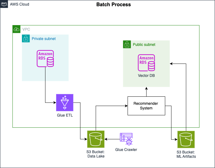
The batch pipeline ingests product and user data from the source database (Amazon RDS MySQL database), transforms it using AWS Glue ETL and stores the transformed data in an Amazon S3 bucket. The data is transformed into training data that will be used by the data scientist to train the recommender system.
Before you implement this pipeline, you will explore an additional table that was added to the
classicmodels MySQL Sample Database
used in Week 2. The additional table is labeled ratings and consists of the ratings assigned
by the users to products they have bought. The ratings are on a scale between 1 to 5
and were generated for this lab.
Exploring the ratings table
The source database (Amazon RDS MySQL database) is already instantiated and
provisioned for you to use in this lab. Let’s connect to it and check the ratings table.
1.1. Get the endpoint (i.e., address) of the database instance with the following command
(replace the <MySQL-DB-name> with de-c1w4-rds):
aws rds describe-db-instances --db-instance-identifier <MySQL-DB-name> --output text --query "DBInstances[].Endpoint.Address"
1.2. Connect to the database by running the following command, replacing
-
<MySQLEndpoint>with the output from the previous step, -
<DatabaseUserName>withadmin, -
<Password>withadminpwrd:
mysql --host=<MySQLEndpoint> --user=<DatabaseUserName> --password=<Password> --port=3306
1.3. Make sure to use the classicmodels database and list the existing tables:
use classicmodels;
show tables;
You should see the new table: ratings.
1.4. To check the first 20 lines of the table, run the following query:
SELECT *
FROM ratings
LIMIT 20;
The LIMIT clause limits the number of rows displayed in the query result,
you can adjust this number to see more or less data.
Try to understand the structure of the ratings table and where it should be placed in the original
schema.
1.5. Quit the connection to the database:
exit
Running AWS Glue ETL Job
You will now create the resources needed for the batch pipeline (AWS Glue ETL and Amazon S3 bucket) using Terraform. Remember that Terraform is an Infrastructures as Code (IaC) tool that allows you to configure and provision resources for your workflow. Once you create the resources, you will run the AWS Glue Job that will ingest the data from RDS and transform it into the training data requested by the data scientist.
1.6. Setup the environment running the script scripts/setup.sh:
source ./scripts/setup.sh
This script installs the necessary packages (PostgreSQL and Terraform) and sets up some environment variables required to pass parameters into the Terraform configuration.
1.7. Go to the terraform folder.
cd terraform
1.8. Open the terraform script terraform/main.tf.
For the part of the batch pipeline, you only have to work on module "etl".
Uncomment the corresponding section of the file (lines 1 to 13), keeping the
rest of the file commented (comments in Terraform start with #).
Note: Remember to save your changes by pressing Ctrl+S or Cmd+S.
1.9. Open the script terraform/outputs.tf and uncomment the lines
corresponding to the ETL section (lines 2 to 8).
Note: Remember to save your changes by pressing Ctrl+S or Cmd+S.
1.10. Initialize the terraform configuration:
terraform init
1.11. To deploy the resources, run the following commands:
terraform plan
terraform apply
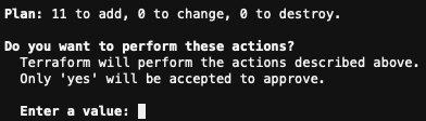
Note: The command terraform apply will prompt you to reply yes here:
1.12. Now that your resources are available, and have been created, go back to the AWS console, search for AWS Glue, and
enter the ETL jobs link on the left panel. You should see a job created
with the name de-c1w4-etl-job.
1.13. Start the AWS Glue job:
aws glue start-job-run --job-name de-c1w4-etl-job | jq -r '.JobRunId'
You should get JobRunID in the output.
1.14. Check the status of the AWS Glue job exchanging the <JobRunID> with the output from the previous step:
aws glue get-job-run --job-name de-c1w4-etl-job --run-id <JobRunID> --output text --query "JobRun.JobRunState"
You can also see the job status in the console by opening the de-c1w4-etl-job
and going to the tab Runs. Wait until the job status changes to
SUCCEEDED (it will take 2-3 min).
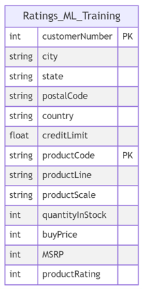
The transformed data has the following schema:
1.15. The AWS Glue Job should transform the data and store it in the data lake S3
bucket that was created with IaC. You can go to the AWS console, search for S3
and then search for a bucket named de-c1w4-<PLACEHOLDER>-datalake.
Under the folder ratings-ml-training you can see some additional
folders with the naming convention: customerNumber=<NUMBER>. This convention
indicates how the data was partitioned during the storage step.
The concept of partitioning will be tackled later in the specialization.
Once the data is there, the ML Team will take this data and train their model.
2 - Creating & Setting up the Vector Database
2.1. Now, let’s suppose the Data Scientist has trained the model. They created the S3 bucket
called de-c1w4-<AWS-ACCOUNT-ID>-us-east-1-ml-artifacts. In that bucket, the Data Scientist
published the results of the model. You can explore the bucket and find the following
folder structure:
.
├── embeddings/
|   ├── item_embeddings.csv
|   └── user_embeddings.csv
├── model/
|   └── best_model.pth
└── scalers/
    ├── item_ohe.pkl
    ├── item_std_scaler.pkl
    ├── user_ohe.pkl
    └── user_std_scaler.pkl
The embeddings folder contains the embeddings of the users and items (or products) that
were generated in the model.
The model folder contains the trained model that will be used for inference.
The scalers folder contains the objects used on the preprocessing part for
the training, such as
One Hot Encoders
and Standard Scalers.
The Data Scientist asked to upload the item_embeddings.csv and user_embeddings.csv
files into a Vector Database (Vector DB). Those embeddings will be used by the
recommender system in the streaming pipeline to provide product recommendations.
The use of a vector database accelerates the retrieval of items that are similar to a
given item. So for example, if a user places an item in the cart, the recommender
model will first compute the embedding vector of this item and then use the vector
database to retrieve similar items to it.
Creating the vector database
For the vector database, you will create with Terraform an RDS PostgreSQL database
with the pgvector extension. The PostgreSQL
database is typically faster for complex queries and data analysis, while MySQL,
which you used previously, is more efficient for simpler queries. Working with Vector
DB PostgreSQL provides more capabilities and flexibility.
2.2. In the Cloud9 environment, open again the /terraform/main.tf
script. Uncomment the module "vector_db" section (lines 15 to 25).
Note: Remember to save your changes by pressing Ctrl+S or Cmd+S.
2.3. In the file /terraform/outputs.tf, uncomment the blocks
associated with the Vector DB (lines 11 to 27).
Note: Remember to save your changes by pressing Ctrl+S or Cmd+S.
2.4. Re-initialize the terraform module, plan and apply changes with the following commands:
terraform init
terraform plan
terraform apply
Note: The command terraform apply will prompt you to reply yes here:
Creation of the database will take around 7 minutes.
2.5. You will see that some information is displayed after the terraform apply
command, but some fields (database username and password) appear as sensitive. In order to see that information,
which will be used to connect to the Vector DB, you need to use the following commands:
terraform output vector_db_master_username
terraform output vector_db_master_password
Save the outputs somewhere locally - you will use them later.
Note: The outputs are printed in double quotes, which are not part of the username or password.
Adding the embeddings to the vector database
Now that the vector database has been created, you will connect to it to import
the embeddings from S3. The sql/embeddings.sql file contains the SQL statements for this task.
2.6. Open the sql/embeddings.sql file and change the bucket placeholders <BUCKET_NAME>
with the de-c1w4-<AWS-ACCOUNT-ID>-us-east-1-ml-artifacts bucket name
(where <AWS-ACCOUNT-ID> is your AWS Account ID). You can go back to step 2.1
to get the bucket name that contains the embeddings.
Note: The change of the bucket placeholders <BUCKET_NAME> should be done in two places!
Note: Remember to save your changes by pressing Ctrl+S or Cmd+S.
2.7. Get the vector_db_host output from Terraform (see the instructions in step 2.5).
You will later use this output, so save it somewhere locally.
2.8. Now connect to the database by running the following command, replacing
<VectorDBHost> with the output from the previous step. You will be asked for a password,
you can use the one obtained in step 2.5.
psql --host=<VectorDBHost> --username=postgres --password --port=5432
2.9. Then, to work in the postgres database use this command with the same password:
\c postgres;
2.10. Once connected to the postgres DB, you can now run the SQL statements
in the script sql/embeddings.sql. Use the following command:
\i '../sql/embeddings.sql'
2.11. To check the available tables, use the following command:
\dt *.*
Press the Q key to quit the psql prompt.
2.12. Quit the psql prompt with the command \q.
Optional: If you’re interested in learning more about postgres flags, you can check link.
3 - Connecting the Deployed Model to the Vector Database
So now you have the vector database created and the embeddings imported inside of it. Let’s see where it fits into the streaming pipeline. Here’s the architectural diagram of the streaming workflow:
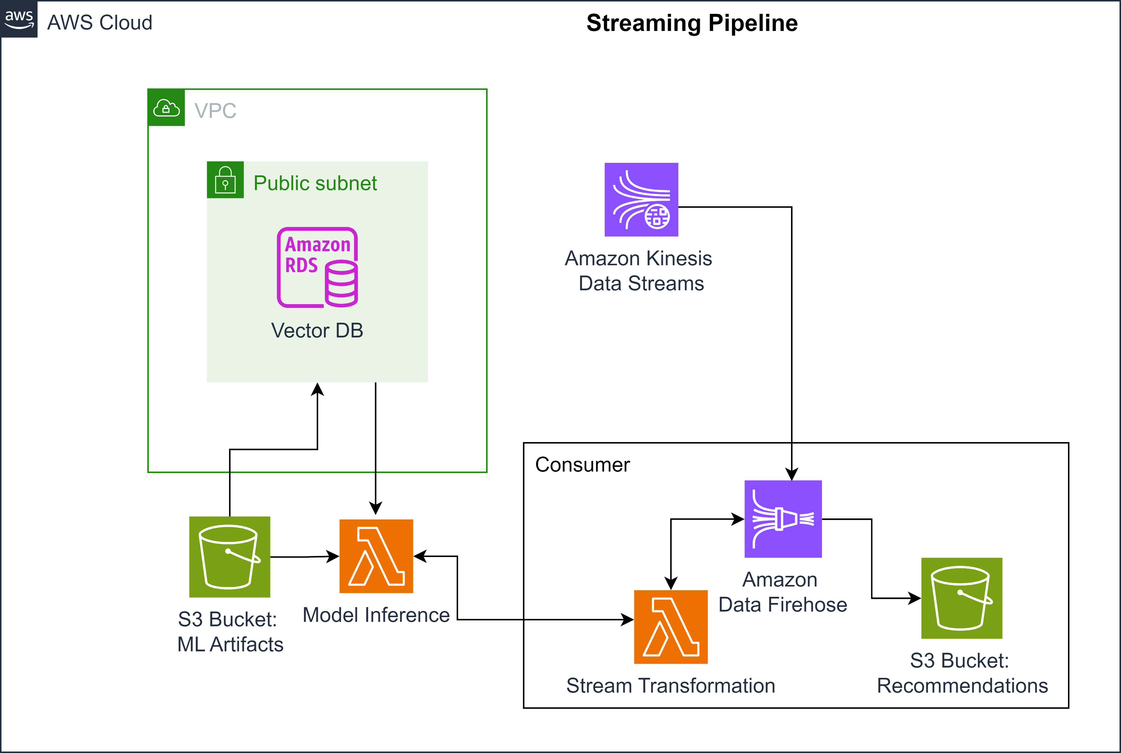
On the left side, you see a lambda function labeled as “model inference”. This lambda function, which is a serverless compute resource, will use the trained model stored in S3 and the embeddings from the vector database to provide the recommendation based on the online user activity streamed by Kinesis Data streams.
In this section, you will configure the variables in the lambda function to make it ready for the streaming pipeline.
3.1. In the AWS Console, search for RDS, click on Databases in the left panel,
and find the database called de-c1w4-vector-db. Click on it.
3.2. In the Connectivity & Security tab, search for the endpoint, which should
have the following structure: de-c1w4-vector-db.xxxxxxxxxxxx.us-east-1.rds.amazonaws.com.
Copy this value and keep it safe as you will use it in a moment
(this is the same endpoint you got with the command terraform output vector_db_host).
3.3. Back to the AWS Console, search for Lambda. Then find again the lambda functionde-c1w4-model-inference.
Click on the name of the lambda and then, scroll down and search for the Configuration tab,
click on it. Then, open Environment Variables from the left panel and click on Edit.
Put the values for the following variables:
-
VECTOR_DB_HOST: VectorDB endpoint that you copied in the previous step, -
VECTOR_DB_PASSWORD: output value from the commandterraform output vector_db_master_password, -
VECTOR_DB_USER: output value from the commandterraform output vector_db_master_username.
Click on Save.
4 - Implementing the Streaming Pipeline
You will now implement the streaming pipeline that consists of Kinesis Data Streams, Kinesis Firehose and S3 (recommendation bucket). Assume that AWS Kinesis Data Streams receives the online user activity from the sales platform log. It then streams this data to Kinesis Data Firehose, which acts as a delivery service that handles loading data streams into S3 (recommendation bucket). Before it loads the data into S3, it invokes the lambda function (stream transformation) that extracts user and product features from the data streams and uses the trained recommender model to find the recommendations and finally, it loads the recommendations into S3 recommendation bucket.
Now use Terraform to create Kinesis Firehose, S3 recommendation bucket, and the lambda function (stream transformation).
4.1. In the Cloud9 environment, open again the /terraform/main.tf script,
uncomment the module "streaming_inference" section (lines 27 to 36).
Note: Remember to save your changes by pressing Ctrl+S or Cmd+S.
4.2. In the file /terraform/outputs.tf, uncomment the blocks associated with the
streaming inference (lines 29 to 32).
Note: Remember to save your changes by pressing Ctrl+S or Cmd+S.
4.3. Re-initialize the terraform module, plan and apply changes:
terraform init
terraform plan
terraform apply
Note: The command terraform apply will prompt you to reply yes.
4.4. Now, back in the AWS Console, search for S3 and click on the recommendation
bucket that was just created using terraform, called de-c1w4-<PLACEHOLDER>-recommendations.
After some time, the Kinesis delivery stream that you created with Firehose will start
consuming data from the Kinesis data stream de-c1w4-kinesis-data-stream.
Then, it will perform the transformations that you set up in the Lambda function
and the S3 bucket will be filled with some files.
You can also go to Lambda and search for de-c1w4-transformation-lambda which
was created with Terraform. Click on it and search the Monitor tab.
Click on View CloudWatch Logs. There you will be able to see the logs of the
function while it performs some transformations. As de-c1w4-kinesis-data-stream
receives data dynamically (with an average time between events of 10 seconds),
the S3 bucket or the Lambda logs can take some minutes to start showing any data
or events. You can wait around 5 minutes and refresh the S3/CloudWatch Logs page
to see the incoming data.
In the S3 bucket, data will be partitioned by date, so you will see a hierarchy of
directories similar to the following:
.
├── year/
    └── month/
        └── day/
            └── hour/
                └── de-c1w4-delivery-stream-<PLACEHOLDER>
In this lab, you went through an end-to-end pipeline for both batch and streaming cases. You built a batch data pipeline with AWS Glue and S3 to provide the training data for the recommender system, you then created a vector database to store the embeddings and finally constructed a real-time streaming pipeline using AWS Kinesis Data Streams and Firehose. And with that, you’ve seen how to translate stakeholder needs into functional and nonfunctional requirements, choose the appropriate tools and then build the data pipeline.